Ikki Ko'rsatkich
Ikki Ko'rsatkich Usuliga Kirish
Ikki Ko'rsatkich Usuliga Kirish
Intuitsiya
Nomidan ko'rinib turibdiki, ikki ko'rsatkich (Two Pointers) namunasi ikkita ko'rsatkichdan foydalanadigan algoritmni anglatadi. Ko'rsatkich nima? Bu massiv yoki bog'liq ro'yxat kabi ma'lumotlar strukturasidagi indeks yoki pozitsiyani ifodalovchi o'zgaruvchi. Ko'plab algoritmlar bitta elementni kuzatish uchun faqat bitta ko'rsatkichdan foydalanadi:
![The image represents a visual depiction of data insertion or modification within a data structure, likely an array or list. A small, orange square containing the letter 'i' acts as an indicator or pointer, positioned above a sequence of numbers enclosed in square brackets: `[ ... 14 5 5 20 ... ]`. A downward-pointing orange arrow originates from the 'i' indicator and points directly to the number '5', suggesting that the 'i' represents a position or index within the data structure, and the arrow indicates the insertion or modification is occurring at that specific index. The ellipses (...) indicate that there are additional elements before and after the visible portion of the sequence. The overall diagram illustrates a simple data manipulation operation, focusing on the insertion or update of a value at a particular index within a larger dataset.](https://bytebytego.com/images/courses/coding-patterns/two-pointers/introduction-to-two-pointers/image-01-00-1-OA7SGCBK.svg?dpl=dpl_Gs7zfM6MUzjTBjcjps1LqXtb9QmD)
Ikkinchi ko'rsatkichni kiritish yangi imkoniyatlar olamini ochadi. Eng muhimi, endi taqqoslashlar qila olamiz. Ikki turli pozitsiyadagi ko'rsatkichlar bilan u pozitsiyadagi elementlarni taqqoslab, natijaga asoslanib qaror qabul qilishimiz mumkin:
![Image represents a visual depiction of a comparison step within a sorting algorithm, likely a comparison-based sort like bubble sort or insertion sort. The diagram shows a numerical array `nums` represented as `[... 14 5 5 20 ...]`, indicating a partial view of a larger array. Two index variables, `i` (in an orange box) and `j` (in a light-blue box), point to elements 14 and 5 respectively within the array. Arrows descend from `i` and `j` to highlight these selected elements. To the right, a dashed-line box describes a function call `compare(nums[i], nums[j])`, which implies a comparison operation between the values at indices `i` and `j` (14 and 5 in this instance). A right-pointing arrow from this box leads to the text 'make decision,' indicating that the result of the comparison (whether `nums[i]` > `nums[j]`, `nums[i]` < `nums[j]`, or `nums[i]` == `nums[j]`) will determine the next step in the sorting algorithm.](https://bytebytego.com/images/courses/coding-patterns/two-pointers/introduction-to-two-pointers/image-01-00-2-Y7CSNC5F.svg?dpl=dpl_Gs7zfM6MUzjTBjcjps1LqXtb9QmD)
Ko'p hollarda bunday taqqoslashlar ikkita ichki for-tsikl yordamida amalga oshiriladi, bu O(n²) vaqt talab qiladi, bu yerda n ma'lumotlar strukturasining uzunligini bildiradi. Quyidagi kod parchasida i va j massivning har ikkita elementini taqqoslash uchun ishlatiladigan ikkita ko'rsatkichdir:
for i in range(n):
    for j in range(i + 1, n):
        compare(nums[i], nums[j])
Ko'pincha bu yondashuv ma'lumotlar strukturasida mavjud bo'lishi mumkin bo'lgan bashorat qilinadigan dinamikadan foydalanmaydi. Bashorat qilinadigan dinamikaga ega ma'lumotlar strukturasiga misol tariqasida tartiblangan massivni keltirish mumkin: tartiblangan massivda ko'rsatkichni siljitganimizda, ko'chirilayotgan qiymat kattami yoki kichikmi ekanini oldindan bilishimiz mumkin. Masalan, o'suvchi massivda ko'rsatkichni o'ngga siljitish joriy qiymatdan katta yoki teng qiymatga o'tishimizni kafolatlaydi:
![Image represents a diagram illustrating a coding pattern or prediction within a sorted array. At the top, a small orange square containing the letter 'i' points downwards, indicating an index or iterator. Below, a sorted integer array `[1 2 3 4]` is shown, with a grey line underneath labeled 'sorted array'. A dashed-line box at the bottom contains a prediction statement written in a pseudo-code style: 'prediction: if nums[i] == 2, then nums[i + 1] ≥ 2'. This statement suggests that if the element at index 'i' in the `nums` array is equal to 2, then the element at the next index (i+1) must be greater than or equal to 2. The arrow from 'i' implies that 'i' is used to index into the array, likely as part of an algorithm or conditional check.](https://bytebytego.com/images/courses/coding-patterns/two-pointers/introduction-to-two-pointers/image-01-00-3-ASETSKFQ.svg?dpl=dpl_Gs7zfM6MUzjTBjcjps1LqXtb9QmD)
Ko'rib turganingizdek, bashorat qilinadigan dinamikaga ega ma'lumotlar strukturalari ko'rsatkichlarni mantiqiy tarzda siljitish imkonini beradi. Bu bashorat qilish qobiliyatidan foydalanish vaqt va xotira murakkabligini yaxshilashga olib keladi, buni bu bobdagi real intervyu masalalari bilan ko'rsatib beramiz.
Ikki Ko'rsatkich Strategiyalari
Ikki ko'rsatkich algoritmlari odatda ichki for-tsikllarni bartaraf etish orqali faqat O(n) vaqt sarflaydi. Ikki ko'rsatkichdan foydalanishning uchta asosiy strategiyasi mavjud.
Ichkariga yo'naltirilgan aylanish Bu yondashuv ko'rsatkichlar ma'lumotlar strukturasining qarama-qarshi uchlaridan boshlanib, bir-biriga qarab ichkariga siljishini nazarda tutadi:
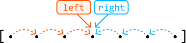
Ko'rsatkichlar ma'lum shart bajarilguncha yoki ular uchrashuv/kesishguncha taqqoslashlar asosida o'z pozitsiyalarini sozlab, markazga qarab siljiydi. Bu ma'lumotlar strukturasining turli uchlaridan elementlarni taqqoslash kerak bo'lgan masalalar uchun ideal.
Bir yo'nalishli aylanish Bu yondashuv ikki ko'rsatkich ham ma'lumotlar strukturasining bir uchidan (odatda boshidan) boshlanib, bir xil yo'nalishda siljishini anglatadi:
![The image represents a visual depiction of a two-pointer approach to traversing a data structure, likely an array or list. The structure is shown as a sequence of black dots enclosed within square brackets `[ ]`, representing individual elements. An orange rectangle labeled 'left' points a downward arrow to the leftmost element within a subset of the dots. Dashed orange lines with arrowheads connect this element to the next few elements to its right, indicating a traversal from left to right. Similarly, a light-blue rectangle labeled 'right' points a downward arrow to the rightmost element within a different subset of the dots. Dashed light-blue lines with arrowheads connect this element to the preceding few elements to its left, indicating a traversal from right to left. The two pointers, indicated by the orange and light-blue arrows, are moving towards the center of the data structure, suggesting a merging or comparison process commonly used in algorithms like merge sort or two-pointer techniques for finding pairs with a specific sum.](https://bytebytego.com/images/courses/coding-patterns/two-pointers/introduction-to-two-pointers/image-01-00-5-2KI3FUD6.svg?dpl=dpl_Gs7zfM6MUzjTBjcjps1LqXtb9QmD)
Bu ko'rsatkichlar odatda ikki xil, lekin to'ldiruvchi maqsadga xizmat qiladi. Buning keng tarqalgan qo'llanilishi — bir ko'rsatkich ma'lumot topishi (odatda o'ng ko'rsatkich) va boshqasi ma'lumotni kuzatib borishi (odatda chap ko'rsatkich) kerak bo'lganda.
Bosqichli aylanish Bu yondashuv bitta ko'rsatkich bilan aylanib, u ma'lum shartga mos keluvchi elementga tushganda ikkinchi ko'rsatkich bilan aylanishni anglatadi:

Bir yo'nalishli aylanishga o'xshab, ikkala ko'rsatkich turli maqsadga xizmat qiladi. Bu yerda birinchi ko'rsatkich biror narsani qidirish uchun ishlatiladi va topilgach, ikkinchi ko'rsatkich birinchi ko'rsatkichdagi qiymatga oid qo'shimcha ma'lumotni topadi.
Biz bu bobdagi masalalar davomida barcha ushbu texnikalarni batafsil muhokama qilamiz.
Ikki Ko'rsatkich Qachon Ishlatiladi?
Ikki ko'rsatkich algoritmi odatda massiv yoki bog'liq ro'yxat kabi chiziqli ma'lumotlar strukturasini talab qiladi. Masalani ikki ko'rsatkich algoritmi yordamida hal qilish mumkinligining ko'rsatkichi — kiritilgan ma'lumotlar tartiblangan massiv kabi bashorat qilinadigan dinamikaga amal qilishi.
Bashorat qilinadigan dinamika ko'p shaklda bo'lishi mumkin. Masalan, palindrom satrni olaylik. Uning simmetrik namunasi ikkita ko'rsatkichni markazga qarab mantiqiy ravishda siljitish imkonini beradi. Bu bobdagi masalalar ustida ishlashingiz davomida ushbu bashorat qilinadigan dinamikani osonroq tanishni o'rganasiz.
Masalani ikki ko'rsatkich yordamida hal qilish mumkinligining yana bir ko'rsatkichi — masala ikki qiymatdan iborat juft yoki ikkita qiymatdan hosil bo'ladigan natijani so'rashi.
Hayotiy Misol
Axlat yig'ish algoritmlari: Xotirani zichlashda — axlat yig'ishning asosiy qismi — maqsad ajratib olingan (ya'ni o'lik) obyektlar qoldirgan bo'shliqlarni bartaraf etib, uzluksiz xotira maydonini bo'shatishdir. Ikki ko'rsatkich texnikasi buni samarali amalga oshirishga yordam beradi: 'skan' ko'rsatkichi tirik obyektlarni aniqlash uchun heap bo'ylab aylanadi, 'bo'sh' ko'rsatkichi esa tirik obyektlar ko'chirilishi kerak bo'lgan keyingi bo'sh joyni kuzatib boradi. 'Skan' ko'rsatkichi siljigan sari o'lik obyektlarni o'tkazib yuboradi va tirik obyektlarni 'bo'sh' ko'rsatkichi ko'rsatgan pozitsiyaga ko'chiradi, barcha tirik obyektlarni birlashtirish va uzluksiz xotira bloklarini bo'shatish orqali xotirani zichlaydi.
Bob Mazmuni
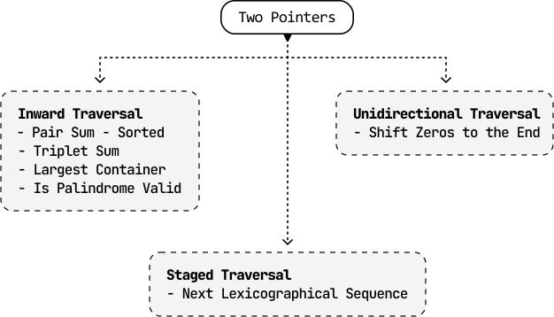
Ikki ko'rsatkich namunasi juda ko'p qirrali va shunga ko'ra ancha keng. Shuning uchun biz Fast and Slow Pointers va Sliding Windows kabi ushbu algoritmning yanada ixtisoslashgan variantlarini alohida boblarda ko'rib chiqmoqchimiz.
Juft Yig'indi - Tartiblangan
Juft Yig'indi - Tartiblangan
O'sish tartibida tartiblangan butun sonlar massivi va maqsad qiymat berilgan, massivda maqsadga teng yig'indili ixtiyoriy son juftining indekslarini qaytaring. Natijedagi indekslar tartibi muhim emas. Agar juft topilmasa, bo'sh massiv qaytaring.
Misol 1:
Input: nums = [-5, -2, 3, 4, 6], target = 7
Output: [2, 3]
Tushuntirish: nums[2] + nums[3] = 3 + 4 = 7
Misol 2:
Input: nums = [1, 1, 1], target = 2
Output: [0, 1]
Tushuntirish: boshqa to'g'ri javoblar [1, 0], [0, 2], [2, 0], [1, 2] yoki [2, 1] bo'lishi mumkin.
Intuitsiya
Ushbu masalaning qo'pol kuch yechimi barcha mumkin bo'lgan juftlarni tekshirishni o'z ichiga oladi. Bu tashqi tsikl juftning birinchi elementi uchun massiv bo'ylab aylanadigan va ichki tsikl ikkinchi elementni topish uchun massivning qolgan qismini aylanadigan ikkita ichki tsikl yordamida amalga oshiriladi. Quyida ushbu yondashuvning kod parchasi:
from typing import List

def pair_sum_sorted_brute_force(nums: List[int], target: int) -> List[int]:
    n = len(nums)
    for i in range(n):
        for j in range(i + 1, n):
            if nums[i] + nums[j] == target:
                return [i, j]
    return []
Bu yondashuvning vaqt murakkabligi O(n²), bu yerda n massiv uzunligini bildiradi. Bu yondashuv kiritilgan massiv tartiblangan ekanini hisobga olmaydi. Bu faktdan foydalanib samaraliroq yechim topishimiz mumkinmi?
Bu yerda ikki ko'rsatkich yondashuvini ko'rib chiqish o'rinli, chunki tartiblangan massiv ko'rsatkichlarni mantiqiy tarzda siljitish imkonini beradi. Quyidagi misolda bu qanday ishlashini ko'rib chiqaylik:
![Image represents a sample input for a coding problem likely related to finding pairs of numbers within an array that sum to a target value. The image shows an integer array `[-5, -2, 3, 4, 6]` enclosed in square brackets, with the index of each element subtly displayed below it (0 through 4). A comma separates the array from the statement 'target = 7,' which specifies the target sum to be found. The arrangement implies that the algorithm should search within the provided array for two numbers that add up to 7. The indices are not explicitly part of the input data but are visually provided to aid understanding of the array's structure.](https://bytebytego.com/images/courses/coding-patterns/two-pointers/pair-sum-sorted/image-01-01-1-GSLVICE3.svg?dpl=dpl_Gs7zfM6MUzjTBjcjps1LqXtb9QmD)
Boshlash uchun eng kichik va eng katta qiymatlarga — mos ravishda birinchi va oxirgi elementlarga — qarash yaxshi joy. Bu ikki qiymatning yig'indisi 1 ga teng.
![Image represents a diagram illustrating a simple summation operation on an array. Two orange rectangular boxes labeled 'left' and 'right' point downwards with arrows towards a numerical array [-5, -2, 3, 4, 6]. The 'left' arrow points to the first two elements of the array, [-5, -2], while the 'right' arrow points to the last three elements, [3, 4, 6]. The array elements are indexed below with numbers 0 through 4, indicating their positions. A separate, light-grey, dashed-line rectangular box displays the result of the summation, showing 'sum = 1'. This implies that the sum of all elements in the array (-5 + -2 + 3 + 4 + 6) equals 1.](https://bytebytego.com/images/courses/coding-patterns/two-pointers/pair-sum-sorted/image-01-01-2-OIIAKQQK.svg?dpl=dpl_Gs7zfM6MUzjTBjcjps1LqXtb9QmD)
1 maqsaddan kichik bo'lgani uchun, kattaroq yig'indili yangi juft topish uchun ko'rsatkichlardan birini siljitishimiz kerak.
- Chap ko'rsatkich: Massiv tartiblanganligi sababli chap ko'rsatkich har doim o'ng ko'rsatkichdagi qiymatdan kichik yoki unga teng qiymatga ishora qiladi. Uni oshirish joriy 1 yig'indisidan katta yoki teng yig'indiga olib keladi.
- O'ng ko'rsatkich: O'ng ko'rsatkichni kamaytirish 1 dan kichik yoki unga teng yig'indiga olib keladi.
Shuning uchun kattaroq yig'indi topish uchun chap ko'rsatkichni oshirishimiz kerak:
![Image represents a visual depiction of a two-pointer algorithm, likely used to find a pair of numbers in a sorted array that sum to a target value (not explicitly shown but implied). The top section shows an initial state with two pointers, labeled 'left' and 'right,' pointing to the beginning and end, respectively, of a sorted array [-5, -2, 3, 4, 6]. The indices (0, 1, 2, 3, 4) are shown below the array elements. A dashed box shows the current sum (1, calculated as -5 + 6) being compared to a target value (7, also implied). Since the sum (1) is less than 7, a solid arrow indicates that the 'left' pointer is incremented (left += 1). The bottom section illustrates the updated state after the pointer increment, where the 'left' pointer now points to -2. The 'right' pointer remains unchanged. The dotted arrow emphasizes the movement of the 'left' pointer. The overall diagram demonstrates a single iteration of the algorithm, highlighting the pointer movement based on the comparison of the current sum with the target value.](https://bytebytego.com/images/courses/coding-patterns/two-pointers/pair-sum-sorted/image-01-01-3-ITV7AUHM.svg?dpl=dpl_Gs7zfM6MUzjTBjcjps1LqXtb9QmD)
Yana, ikkita ko'rsatkichdagi qiymatlarning yig'indisi (4) juda kichik. Shuning uchun chap ko'rsatkichni oshiraylik:
![Image represents a visual depiction of a coding pattern, likely illustrating a two-pointer approach or a similar algorithm operating on an array. The top section shows an array `[-5, -2, 3, 4, 6]` with pointers labeled 'left' and 'right' initially pointing to the first and last elements respectively. The indices of the array elements are shown below the array. A dashed box displays a condition: `sum = 4 < 7`, indicating that the sum of elements pointed to by 'left' (3) and 'right' (6) is 4, which is less than 7. A thick arrow connects this condition to another dashed box showing the consequence: `left += 1`, signifying that the 'left' pointer is incremented. The bottom section shows the state after this operation: the 'left' pointer has moved one position to the right, now pointing to the element 3, while the 'right' pointer remains unchanged. The 'left' pointer in the bottom section is highlighted in orange to emphasize its movement. The overall diagram illustrates a step-by-step execution of a code segment that iterates through an array, potentially searching for a specific condition or performing a calculation based on the values pointed to by the 'left' and 'right' pointers.](https://bytebytego.com/images/courses/coding-patterns/two-pointers/pair-sum-sorted/image-01-01-4-5EETAG3M.svg?dpl=dpl_Gs7zfM6MUzjTBjcjps1LqXtb9QmD)
Endi yig'indi (9) juda katta. Shuning uchun kichikroq yig'indili qiymatlar juftini topish uchun o'ng ko'rsatkichni kamaytirishimiz kerak:
![Image represents a visual depiction of a coding pattern, possibly illustrating a segment of an algorithm. The top section shows an array `[-5, -2, 3, 4, 6]` with indices 0 through 4 labeled below. Above the array, two rectangular boxes labeled 'left' and 'right' point downwards, indicating pointers or indices. The 'left' pointer points to the element '3' (index 2), and the 'right' pointer points to the element '6' (index 4). A dashed box to the right shows a calculation: 'sum = 9 > 7', implying the sum of the elements pointed to by 'left' and 'right' (3 + 6 = 9) is greater than 7. An arrow then points to another box indicating 'right -= 1', suggesting the 'right' pointer's index is decremented. The bottom section shows the updated state after this operation. The array remains the same, but the 'right' pointer (now orange) points to the element '4' (index 3), illustrating the effect of the decrement operation. A dotted line shows the movement of the 'right' pointer from index 4 to index 3. The 'left' pointer remains unchanged.](https://bytebytego.com/images/courses/coding-patterns/two-pointers/pair-sum-sorted/image-01-01-5-UOKAUU5C.svg?dpl=dpl_Gs7zfM6MUzjTBjcjps1LqXtb9QmD)
Nihoyat, maqsadga teng yig'indi beradigan ikkita son topdik. Ularning indekslarini qaytaylik:
![Image represents a diagram illustrating a coding pattern, possibly related to array processing or a divide-and-conquer algorithm. At the top, two orange rectangular boxes labeled 'left' and 'right' are shown. Arrows descend from these boxes, pointing to the elements '3' and '4' respectively, within a horizontal array represented as `[-5, -2, 3, 4, 6]`. The array indices (0, 1, 2, 3, 4) are displayed beneath the corresponding array elements. A light gray, dashed-bordered rectangle contains the expression 'sum = 7 == 7', indicating a comparison where the sum of some values (implied to be '3' and '4') equals 7. A thick arrow points from this comparison to the text 'return [left, right]', suggesting that if the comparison is true, the function returns an array containing the values 'left' and 'right'. The overall diagram visually depicts the process of selecting elements from an array based on some condition (here, implicitly the sum of selected elements), and returning a result based on those selections.](https://bytebytego.com/images/courses/coding-patterns/two-pointers/pair-sum-sorted/image-01-01-6-C3CZ7WBU.svg?dpl=dpl_Gs7zfM6MUzjTBjcjps1LqXtb9QmD)
Yuqorida biz ichkariga yo'naltirilgan aylanishdan foydalanadigan ikki ko'rsatkich algoritmini ko'rsatdik. Keling, bu mantiqni xulosalaymiz. Chap va o'ngdagi ixtiyoriy qiymatlar jufti uchun:
- Agar ularning yig'indisi maqsaddan kichik bo'lsa, yig'indini maqsad qiymatga yaqinlashtirish maqsadida chapni oshiring.
- Agar ularning yig'indisi maqsaddan katta bo'lsa, yig'indini maqsad qiymatga yaqinlashtirish maqsadida o'ngni kamaytiring.
- Agar ularning yig'indisi maqsad qiymatga teng bo'lsa, [left, right] qaytaring.
Chap va o'ng ko'rsatkichlar uchrashuv paytida ularni siljitishni to'xtatishimiz mumkin, chunki bu maqsadga yig'indilovchi juft topilmaganligini bildiradi.
Amalga oshirish
from typing import List

def pair_sum_sorted(nums: List[int], target: int) -> List[int]:
    left, right = 0, len(nums) - 1
    while left < right:
        sum = nums[left] + nums[right]
        # If the sum is smaller, increment the left pointer, aiming to increase the
        # sum towards the target value.
        if sum < target:
            left += 1
        # If the sum is larger, decrement the right pointer, aiming to decrease the
        # sum towards the target value.
        elif sum > target:
            right -= 1
        # If the target pair is found, return its indexes.
        else:
            return [left, right]
    return []
Murakkablik Tahlili
Vaqt murakkabligi: pair_sum_sorted ning vaqt murakkabligi O(n), chunki eng yomon holatda ikki ko'rsatkich texnikasidan foydalanib taxminan n ta iteratsiya bajaramiz.
Xotira murakkabligi: Biz faqat doimiy sondagi o'zgaruvchilar ajratdik, shuning uchun xotira murakkabligi O(1).
Test Holatlari
Allaqachon muhokama qilingan misollarga qo'shimcha ravishda, quyida foydalanishingiz mumkin bo'lgan boshqa test holatlari keltirilgan. Bu qo'shimcha test holatlari kodni turli kiritish qiymatlari bo'ylab yaxshi ishlashini ta'minlash uchun turli kontekstlarni qamrab oladi. Sinov muhim, chunki u koddagi xatolarni aniqlashga yordam beradi, yechim noodatiy kiritish qiymatlari uchun ham ishlashini ta'minlaydi va siz e'tibordan chetda qoldirgan holatlarga diqqatni qaratadi.
| Input | Expected output | Description |
|---|---|---|
nums = [] target = 0 | [] | Tests an empty array. |
nums = [1] target = 1 | [] | Tests an array with just one element. |
nums = [2, 3] target = 5 | [0, 1] | Tests a two-element array that contains a pair that sums to the target. |
nums = [2, 4] target = 5 | [] | Tests a two-element array that doesn’t contain a pair that sums to the target. |
nums = [2, 2, 3] target = 5 | [0, 2] or [1, 2] | Testing an array with duplicate values. |
nums = [-1, 2, 3] target = 2 | [0, 2] | Tests if the algorithm works with a negative number in the target pair. |
nums = [-3, -2, -1] target = -5 | [0, 1] | Tests if the algorithm works with both numbers of the target pair being negative. |
Intervyu Maslahat
Maslahat: Barcha berilgan ma'lumotlarni hisobga oling. Intervyu olib boruvchilar masala qo'yganlarida, ba'zan uni hal qilishni boshlash uchun kerakli minimal miqdordagi ma'lumotni taqdim etadilar. Shuning uchun masalani samarali hal qilish uchun qaysi tafsilotlar muhimligini aniqlash maqsadida barcha ma'lumotlarni to'liq baholash juda muhim. Ushbu masalada optimal yechimga erishishning kaliti kiritilgan ma'lumotlar tartiblangan ekanligini tan olishdir.
Uchlik Yig'indi
Uchlik Yig'indi
Butun sonlar massivi berilgan, a + b + c = 0 bo'ladigan barcha [a, b, c] uchliklarini qaytaring. Yechim takroriy uchliklarni o'z ichiga olmasligi kerak (masalan, [1, 2, 3] va [2, 3, 1] takroriy hisoblanadi). Agar bunday uchliklar topilmasa, bo'sh massiv qaytaring.
Har bir uchlik ixtiyoriy tartibda joylashtirilishi mumkin va chiqish ixtiyoriy tartibda qaytarilishi mumkin.
Misol:
Input: nums = [0, -1, 2, -3, 1]
Output: [[-3, 1, 2], [-1, 0, 1]]
Intuitsiya
Qo'pol kuch yechimi massivdagi har bir mumkin bo'lgan uchlikni nolga teng yig'indi berish-bermasligini tekshirishni o'z ichiga oladi. Bu uchta elementning har bir kombinatsiyasini takrorlab o'tuvchi uchta ichki tsikl yordamida amalga oshirilishi mumkin.
Takroriy uchliklardan qochish mumkin, har bir uchlikni tartiblash orqali turli tartibdagi bir xil uchliklarning (masalan, [1, 3, 2] va [3, 2, 1]) bir xil tartibda bo'lishini ta'minlash (masalan, [1, 2, 3]). Tartiblanganidan so'ng, bu uchliklarni hash to'plamiga qo'shishimiz mumkin. Shunday qilib, bir xil uchlik yana uchratilsa, hash to'plam faqat bitta nusxani saqlaydi. Quyida ushbu yondashuvning kod parchasi:
from typing import List

def triplet_sum_brute_force(nums: List[int]) -> List[List[int]]:
    n = len(nums)
    # Use a hash set to ensure we don't add duplicate triplets.
    triplets = set()
    # Iterate through the indexes of all triplets.
    for i in range(n):
        for j in range(i + 1, n):
            for k in range(j + 1, n):
                if nums[i] + nums[j] + nums[k] == 0:
                    # Sort the triplet before including it in the hash set.
                    triplet = tuple(sorted([nums[i], nums[j], nums[k]]))
                    triplets.add(triplet)
    return [list(triplet) for triplet in triplets]
Bu yechim vaqt murakkabligi O(n³) bo'lgan juda samarasiz, bu yerda n kiritilgan massiv uzunligini bildiradi. Buni qanday yaxshilash mumkin?
Keling, 0 ga yig'indisi bo'lgan kamida bitta uchlikni topa olamizmi, ko'rib chiqaylik. Agar uchlikdagi sonlardan birini belgilasak, masalani boshqa ikkitasini topishga qisqartirish mumkin ekanligiga e'tibor bering. Bu quyidagi kuzatuvga olib keladi:
Ixtiyoriy [a, b, c] uchligi uchun, agar 'a' ni belgilasak, '-a' ga teng yig'indili [b, c] juftini topishga e'tibor qaratishimiz mumkin (a + b + c = 0 → b + c = -a).
Tanish tuyulyaptimi? Chunki maqsadga teng yig'indili son juftini topish masalasi allaqachon Juft Yig'indi - Tartiblangan tomonidan hal qilingan. Lekin biz bu algoritmni faqat tartiblangan massivda ishlata olamiz. Shuning uchun birinchi qilishimiz kerak bo'lgan narsa kiritilgan ma'lumotni tartiblashdir. Quyidagi misolni ko'rib chiqing:
![Image represents a visual depiction of a sorting operation. The image shows an unsorted array `[-1, 2, -2, 1, -1, 2]` enclosed in square brackets on the left. A rightward-pointing arrow labeled 'sort' connects this initial array to a second array `[-2, -1, -1, 1, 2, 2]` also enclosed in square brackets on the right. The arrow indicates the transformation of the input array (on the left) into the sorted output array (on the right) using a sorting algorithm (implied by the label 'sort'). The numbers within each array represent the elements of the array, and their order demonstrates the before-and-after effect of the sorting process. The output array shows the elements of the input array arranged in ascending order.](https://bytebytego.com/images/courses/coding-patterns/two-pointers/triplet-sum/image-01-02-1-A36R4A4P.svg?dpl=dpl_Gs7zfM6MUzjTBjcjps1LqXtb9QmD)
Endi birinchi element -2 dan (ya'ni 'a') boshlab, massivning qolgan qismida yig'indisi 2 ga (ya'ni '-a') teng juft topish uchun pair_sum_sorted metodidan foydalanamiz:
![Image represents a visual depiction of the `pair_sum_sorted` function's execution on a sorted array `[-2, -1, -1, 1, 2, 2]`, aiming to find triplets summing to a target of 2. The top shows the input array `a` labeled with 'i' indicating an index. An arrow points downwards to the function call `pair_sum_sorted([-1, -1, 1, 2, 2], target = 2)`, excluding the initial -2. The function iteratively uses two pointers, `left` and `right`, initially pointing to the first and last elements of the sub-array, respectively. Each step shows the current array section, the positions of `left` and `right` highlighted in orange boxes, the calculated `sum` of the elements at these positions, and the resulting adjustment to `left` or `right` based on whether the `sum` is less than, greater than, or equal to the target. The process continues until `left` and `right` cross, at which point 'no pairs found' is indicated, implying no triplet starting with -2 sums to 2. Finally, a concluding statement 'no triplet exists that starts with -2' summarizes the function's outcome.](https://bytebytego.com/images/courses/coding-patterns/two-pointers/triplet-sum/image-01-02-2-GBLVHF4M.svg?dpl=dpl_Gs7zfM6MUzjTBjcjps1LqXtb9QmD)
Ko'rib turganingizdek, pair_sum_sorted chaqirilganda, yig'indisi 2 ga teng juft topmadik. Bu -2 dan boshlanadigan, 0 ga qo'shiladigan uchliklar yo'qligini bildiradi.
Shuning uchun asosiy ko'rsatkichimiz i ni oshirib, qayta urinib ko'raylik.
![Image represents a flowchart illustrating the `pair_sum_sorted` algorithm. The algorithm starts with a sorted input array `[-2, -1, -1, 1, 2, 2]` labeled 'a'. The function `pair_sum_sorted([-1, 1, 2, 2], target = 1)` is then called, indicating a search for pairs summing to 1 within the sub-array `[-1, 1, 2, 2]`. Two pointers, `left` and `right`, initially point to the first and last elements of this sub-array respectively. The algorithm iteratively checks the sum of the elements pointed to by `left` and `right`. If the sum equals the target (1), a pair is found ([-1, 2], labeled 'b' and 'c'), and `left` is incremented to find more pairs. If the sum is greater than the target, `right` is decremented. If the sum is less than the target, `left` is incremented (not explicitly shown but implied). This process continues until `left` and `right` cross, at which point the algorithm terminates. The final result, pairs found `[-1, 2]`, is shown, along with a note indicating how these pairs are added to a result array. The flowchart visually depicts the flow of control and data manipulation within the algorithm, showing the changes in pointer positions and the conditional logic based on the sum of the elements.](https://bytebytego.com/images/courses/coding-patterns/two-pointers/triplet-sum/image-01-02-3-XR7EOGIZ.svg?dpl=dpl_Gs7zfM6MUzjTBjcjps1LqXtb9QmD)
Bu safar to'g'ri uchlikka olib keladigan bitta juft topdik.
Agar biz bu jarayonni massivning qolgan qismi uchun davom ettirsak, [-1, -1, 2] yig'indisi 0 bo'lgan yagona uchlik ekanligini aniqlaymiz.
Juft Yig'indi - Tartiblangan dagi pair_sum_sorted amalga oshirilishi va ushbu masaladagi orasida muhim farq bor: bu masala uchun bitta juft topganimizda to'xtatmaymiz, barcha maqsadli juftlar topilguncha davom ettiramiz.
Takroriy uchliklarni boshqarish Biz oldin e'tibordan chetda qoldirgan narsa — takroriy uchliklarni qo'shishdan qanday qochish. Buning ikkita holati mavjud. Quyidagi misolni ko'rib chiqing:

1-holat: takroriy 'a' qiymatlari
Takroriylar yuzaga kelishi mumkin bo'lgan birinchi holat — bir xil 'a' qiymatidan boshlanadigan uchliklar uchun juftlarni qidirish paytida:
![Image represents two identical examples of a data transformation process. Each example shows a sequence of numbers arranged into three labeled groups: 'a', 'b', and 'c'. Group 'a' contains the numbers [-4, -4, -2, 0], group 'b' contains [0, 1, 2], and group 'c' contains [3]. A rightward arrow indicates a transformation where the first element from each group ('a', 'b', and 'c') – specifically -4, 0, and 3 – are extracted and combined to form a new data structure labeled 'triplet [-4 1 3]'. The arrangement is replicated identically below the first example, emphasizing the consistent application of the transformation rule. The labels 'a', 'b', and 'c' are consistently placed above their respective number groups in both examples.](https://bytebytego.com/images/courses/coding-patterns/two-pointers/triplet-sum/image-01-02-5-TXGNCZDQ.svg?dpl=dpl_Gs7zfM6MUzjTBjcjps1LqXtb9QmD)
pair_sum_sorted ikkala holatda ham '-a' ga yig'indili juftlarni qidirganligi sababli, biz tabiiy ravishda bir xil juftlarga va shuning uchun bir xil uchliklariga kelib qolardik.
Bir xil 'a' qiymatini tanlamaslik uchun, i ni (bu yerda nums[i] 'a' qiymatini ifodalaydi) oldingi sondan farqli songa yetguncha oshirib boramiz. Buni pair_sum_sorted metodi yordamida juftlarni qidirishni boshlashdan oldin qilamiz. Bu mantiq ishlaydi, chunki massiv tartiblangan, ya'ni teng sonlar bir-birining yonida. 'a' qiymatlarining takrorlarini tekshirish uchun kod parchasi quyidagicha:
# To prevent duplicate triplets, ensure 'a' is not a repeat of the previous element
# in the sorted array.
if i > 0 and nums[i] == nums[i - 1]:
    continue
... Find triplets ...
2-holat: takroriy 'b' qiymatlari
Ikkinchi holat uchun, o'xshash muammoga duch kelganimizda pair_sum_sorted paytida nima sodir bo'lishini ko'rib chiqing. Belgilangan maqsad qiymat ('-a') uchun, bir xil 'b' sonidan boshlanadigan juftlar har doim bir xil bo'ladi:
![Image represents two examples of extracting a triplet from a larger array. Each example shows a numerical array enclosed in square brackets, containing the elements [-4, -4, -2, 0, 0, 1, 2, 3]. Above each element within the array, labels 'a', 'b', and 'c' are placed to identify sections. In both examples, a sub-array consisting of three elements is highlighted with a cyan-colored box. The first example highlights the elements 0, 0, and 1 (labeled b, b, and c respectively), while the second example highlights the elements 0, 0, and 1 (labeled a, b, and c respectively). A rightward arrow connects each array to the resulting 'triplet,' which is represented as [-2, 0, 2] in both cases. Note that the triplet's values are not directly taken from the highlighted sub-array but rather seem to be a result of some transformation or operation not explicitly shown in the diagram.](https://bytebytego.com/images/courses/coding-patterns/two-pointers/triplet-sum/image-01-02-6-Z75F3BAY.svg?dpl=dpl_Gs7zfM6MUzjTBjcjps1LqXtb9QmD)
Buning davo usuli avvalgidek: joriy 'b' qiymati oldingi qiymatdan farqli ekanligini ta'minlang.
E'tiborli narsa shuki, 'c' qiymatlarining takrorlarini aniq boshqarishimiz shart emas. 'a' va 'b' qiymatlarining takrorlaridan qochish uchun amalga oshirilgan tuzatishlar har bir [a, b] juftining noyob ekanligini ta'minlaydi. 'c' c = -(a + b) tenglamasi bilan aniqlanganligidan, har bir noyob [a, b] jufti noyob 'c' qiymatiga olib keladi. Shuning uchun, faqat 'a' va 'b' dagi takrorlardan qochish orqali [a, b, c] uchliklaridagi takrorlardan avtomatik ravishda qochamiz.
Optimizatsiya Qiziqarli kuzatuv shundan iboratki, faqat musbat sonlardan 0 ga yig'indilaydigan uchliklar hosil qilib bo'lmaydi. Shuning uchun, musbat 'a' qiymatiga yetganimizda uchlik qidirishni to'xtatishimiz mumkin, chunki bu 'b' va 'c' ham musbat bo'lishini anglatadi.
Amalga oshirish
Yuqoridagi intuitsiyadan biz takroriy uchliklardan qochish uchun pair_sum_sorted funksiyasini biroz o'zgartirish kerakligini bilamiz. Biz shuningdek juft-yig'indi algoritmini bajarmoqchi bo'lgan quyi massivning boshini ko'rsatish uchun boshlang'ich qiymatni uzatishimiz kerak. Aks holda, ikki ko'rsatkich mantiqi Juft Yig'indi - Tartiblangan mantig'iga deyarli o'xshash bo'lib qoladi.
from typing import List

def triplet_sum(nums: List[int]) -> List[List[int]]:
    triplets = []
    nums.sort()
    for i in range(len(nums)):
        # Optimization: triplets consisting of only positive numbers will never sum
        # to 0.
        if nums[i] > 0:
            break
        # To avoid duplicate triplets, skip 'a' if it's the same as the previous
        # number.
        if i > 0 and nums[i] == nums[i - 1]:
            continue
        # Find all pairs that sum to a target of '-a' ('-nums[i]').
        pairs = pair_sum_sorted_all_pairs(nums, i + 1, -nums[i])
        for pair in pairs:
            triplets.append([nums[i]] + pair)
    return triplets

def pair_sum_sorted_all_pairs(nums: List[int], start: int, target: int) -> List[int]:
    pairs = []
    left, right = start, len(nums) - 1
    while left < right:
        sum = nums[left] + nums[right]
        if sum == target:
            pairs.append([nums[left], nums[right]])
            left += 1 # To avoid duplicate '[b, c]' pairs, skip 'b' if it’s the same as the # previous number.
            while left < right and nums[left] == nums[left - 1]:
                left += 1
        elif sum < target:
            left += 1
        else:
            right -= 1
    return pairs
Murakkablik Tahlili
Vaqt murakkabligi: triplet_sum ning vaqt murakkabligi O(n²). Sababi:
- Biz avval massivni tartiblashimiz kerak, bu O(n log(n)) vaqt oladi.
- Keyin, massivdagi har bir n element uchun pair_sum_sorted_all_pairs ni ko'pi bilan bir marta chaqiramiz, bu O(n) vaqtda ishlaydi.
Shuning uchun umumiy vaqt murakkabligi O(log(n)) + O(n²) = O(n²) ni tashkil etadi.
Xotira murakkabligi: Xotira murakkabligi Python ning tartiblash algoritmi tomonidan egallangan joyga ko'ra O(n) ni tashkil etadi. Ushbu murakkablik chiqish massivi uchliklarini o'z ichiga olmasligini ta'kidlash muhim, chunki biz faqat algoritm tomonidan ishlatiladigan qo'shimcha joyni, chiqish uchun kerakli joyni emas, nazarda tutamiz.
Agar intervyu olib boruvchi chiqish massivini qo'shsak xotira murakkabligi qanday bo'lishi haqida so'rasa, u O(n²) bo'ladi. Buning sababi, pair_sum_sorted_all_pairs funksiyasi eng yomon holatda chiqishga taxminan n juft qo'shishi mumkin. Bu funksiya taxminan n marta chaqirilganligidan, umumiy xotira murakkabligi O(n²) ni tashkil etadi.
Test Holatlari
Ushbu tushuntirish doirasida allaqachon ko'rib chiqilgan misollarga qo'shimcha ravishda, quyida kodingizni sinash paytida ko'rib chiqiladigan boshqalar keltirilgan.
| Input | Expected output | Description |
|---|---|---|
nums = [] | [] | Tests an empty array. |
nums = [0] | [] | Tests a single-element array. |
nums = [1, -1] | [] | Tests a two-element array. |
nums = [0, 0, 0] | [0, 0, 0] | Tests an array where all three of its values are the same. |
nums = [1, 0, 1] | [] | Tests an array with no triplets that sum to 0. |
nums = [0, 0, 1, -1, 1, -1] | [-1, 0, 1] | Tests an array with duplicate triplets. |
Palindrom Haqiqiyligini Tekshirish
Palindrom Haqiqiyligini Tekshirish
Palindrom — oldinga ham, orqaga ham bir xil o'qiladigan belgilar ketma-ketligi.
Satr berilgan, barcha alifbodan tashqari belgilarni olib tashlaganidan keyin palindrom ekanligini aniqlang. Harf yoki son bo'lsa, belgi alifboviy-raqamli hisoblanadi.
Misol 1:
Input: s = 'a dog! a panic in a pagoda.'
Output: True
Misol 2:
Input: s = 'abc123'
Output: False
Cheklovlar:
- Satr kichik harfli ingliz harflari, sonlar, bo'shliqlar va tinish belgilarining kombinatsiyasini o'z ichiga olishi mumkin.
Intuitsiya
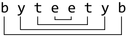
Palindromlarni aniqlash Satr chapdan o'ngga va o'ngdan chapga o'qilganda bir xil bo'lsa, u palindromdir.

Muhim kuzatuv shundan iboratki, agar satr palindrom bo'lsa, birinchi belgi oxirgi belgi bilan bir xil bo'ladi.
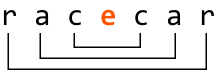
Toq uzunlikdagi palindrom farqli, chunki u o'rta belgiga ega. Bu holda o'rta belgi har qanday belgi bo'lishi mumkin.
Palindromlar ikki ko'rsatkich (chap va o'ng) dan foydalanish uchun ideal shart yaratadi. Dastlab ko'rsatkichlarni satrning ikki uchiga qo'yib:
- Agar chap va o'ngdagi alifboviy-raqamli belgilar bir xil bo'lsa, keyingi juftni qayta ishlash uchun ikkala ko'rsatkichni ichkariga siljiting.
- Aks holda, satr palindrom emas: false qaytaring.
Agar false qaytarmasdan barcha belgi juftlarini muvaffaqiyatli taqqoslasak, satr palindromdir va true qaytaramiz.
Alifbodan tashqari belgilarni qayta ishlash Endi alifbodan tashqari belgilarni o'z ichiga olgan palindromlarni qanday topishni ko'rib chiqaylik.
Alifbodan tashqari belgilar satrnning palindrom ekanligiga ta'sir qilmasligi sababli ularni o'tkazib yuborishimiz kerak.
- Chap ko'rsatkich to'g'rilaydigan belgisi alifboviy-raqamli bo'lguncha uni oshiring.
- O'ng ko'rsatkich to'g'rilaydigan belgisi alifboviy-raqamli bo'lguncha uni kamaytiring.
Shu ma'lumotlardan foydalanib, quyidagi satrning palindrom ekanligini tekshiraylik.
![Image represents a diagram illustrating a coding pattern, possibly related to array or string manipulation. Two orange rectangular boxes labeled 'left' and 'right' are positioned above a line of text 'a + 2 c ! 2 a'. Arrows descend from each box, pointing to the respective ends of this text string. Below, a light-grey, dashed-bordered rectangle contains the conditional statement 's[left] == s[right]', which checks for equality between elements at indices 'left' and 'right' of an array or string 's'. A right-pointing arrow follows this condition, leading to the consequent action 'left += 1, right -= 1', indicating that the 'left' index is incremented and the 'right' index is decremented. The overall diagram suggests an algorithm that iterates through a sequence from both ends, comparing elements until a mismatch is found or the indices cross.](https://bytebytego.com/images/courses/coding-patterns/two-pointers/is-palindrome-valid/image-01-03-4-G3VSN7L3.svg?dpl=dpl_Gs7zfM6MUzjTBjcjps1LqXtb9QmD)
![Image represents a diagram illustrating a coding pattern. At the top, two orange rectangular boxes labeled 'left' and 'right' are shown. A downward-pointing arrow extends from each box. Below the boxes, a string 'a + 2 c ! 2 a' is displayed. The 'left' arrow points to the 'a + 2' portion of the string, and the 'right' arrow points to the 'c ! 2 a' portion. A light gray, dashed-bordered rectangle contains the text 's[left] is not alphanumeric → left += 1,' indicating a conditional statement. This statement checks if the character at the index specified by the variable `left` within string `s` is not alphanumeric. If the condition is true, the value of `left` is incremented by 1. The arrow within the gray rectangle visually represents the flow of control based on the condition's outcome.](https://bytebytego.com/images/courses/coding-patterns/two-pointers/is-palindrome-valid/image-01-03-5-GULODSHO.svg?dpl=dpl_Gs7zfM6MUzjTBjcjps1LqXtb9QmD)
![Image represents a diagram illustrating a coding pattern, possibly related to string manipulation or array processing. At the top, two orange rectangular boxes labeled 'left' and 'right' are shown. Arrows descend from each box pointing to a string 'a + 2 c ! 2 a'. This string appears to be the input data, with 'left' pointing to the 'a + 2' segment and 'right' pointing to the '2 a' segment. Below the input string, a light gray, dashed-bordered rectangle contains the core logic: 's[left] == s[right] → left += 1, right -= 1'. This expression signifies a comparison: if the element at index 'left' in string 's' is equal to the element at index 'right', then the 'left' index is incremented by 1, and the 'right' index is decremented by 1. This suggests an algorithm that iterates from both ends of the string, comparing elements until a mismatch is found or the indices cross. The arrow ('→') indicates the conditional action taken upon successful comparison.](https://bytebytego.com/images/courses/coding-patterns/two-pointers/is-palindrome-valid/image-01-03-6-OXZ53ZN2.svg?dpl=dpl_Gs7zfM6MUzjTBjcjps1LqXtb9QmD)
![Image represents a diagram illustrating a coding pattern, specifically a conditional assignment. At the top, two rectangular boxes labeled 'left' and 'right' (in orange) are shown. Downward arrows from these boxes point to a string 'a + 2 c ! 2 a'. This string appears to represent an input, with 'left' pointing to 'a + 2 c' and 'right' pointing to '! 2 a'. Below this, a light gray, dashed-bordered rectangle contains the conditional statement: 's[right] is not alphanumeric → right -= 1'. This statement indicates that if the substring referenced by `s[right]` (which is '! 2 a' in this example) is not alphanumeric, then the value of the variable `right` is decremented by 1. The arrow ('→') signifies the conditional flow, showing the consequence of the condition being met. The diagram visually demonstrates how the 'right' variable's value might change based on the content of the input string.](https://bytebytego.com/images/courses/coding-patterns/two-pointers/is-palindrome-valid/image-01-03-7-FCOFJ4R5.svg?dpl=dpl_Gs7zfM6MUzjTBjcjps1LqXtb9QmD)

Yuqorida ko'rsatilganidek, chap va o'ng ko'rsatkichlar uchrashuv paytida chiqish sharti bajariladi. Bu ko'rsatkichlar uchrashuv paytida, barcha juftlarni muvaffaqiyatli taqqoslaganimizdan so'ng, true qaytarish vaqti keladi.
![Image represents a diagram illustrating a coding pattern, possibly related to string manipulation or palindrome checking. At the top, two orange rectangular boxes labeled 'left' and 'right' are shown. Arrows point downwards from these boxes to a sequence of characters 'a b b a' below. This sequence appears to be a string being processed. A light gray, dashed-bordered rectangle contains the core logic: 's[left] == s[right] → left += 1, right -= 1'. This expression indicates a comparison: the character at index `left` in string `s` is compared to the character at index `right`. If they are equal (indicated by '=='), then the `left` index is incremented by 1 ('left += 1') and the `right` index is decremented by 1 ('right -= 1'). This suggests an iterative approach, moving inwards from both ends of the string, likely to check for palindromic properties. The arrow ('→') signifies the conditional execution of the index updates based on the comparison result.](https://bytebytego.com/images/courses/coding-patterns/two-pointers/is-palindrome-valid/image-01-03-9-URNCPQKB.svg?dpl=dpl_Gs7zfM6MUzjTBjcjps1LqXtb9QmD)
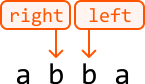
Shuning uchun, chap o'ngga teng yoki uni o'tkazib ketganda tsikldan chiqishimizni ta'minlashimiz kerak. Bu false qaytarmasdan barcha belgi juftlarini taqqoslaganimizni bildiradi va satr palindromdir.
while left < right:
Amalga oshirish
Python da belgining alifboviy-raqamli ekanligini tekshirish uchun o'rnatilgan isalnum metodidan foydalanishimiz mumkin.
def is_palindrome_valid(s: str) -> bool:
    left, right = 0, len(s) - 1
    while left < right:
        # Skip non-alphanumeric characters from the left.
        while left < right and not s[left].isalnum():
            left += 1
        # Skip non-alphanumeric characters from the right.
        while left < right and not s[right].isalnum():
            right -= 1
        # If the characters at the left and right pointers don’t match, the string is
        # not a palindrome.
        if s[left] != s[right]:
            return False
        left += 1
        right -= 1
    return True
Murakkablik Tahlili
Vaqt murakkabligi: is_palindrome_valid ning vaqt murakkabligi O(n), bu yerda n satr uzunligini bildiradi.
Xotira murakkabligi: Biz faqat doimiy sondagi o'zgaruvchilar ajratdik, shuning uchun xotira murakkabligi O(1).
Test Holatlari
Muhokama qilingan misollarga qo'shimcha ravishda, quyida kodingizni sinash paytida ko'rib chiqiladigan ko'proq misollar keltirilgan.
| Input | Expected output | Description |
|---|---|---|
s = "" | True | Tests an empty string. |
s = "a" | True | Tests a single-character string. |
s = "aa" | True | Tests a palindrome with two characters. |
s = "ab" | False | Tests a non-palindrome with two characters. |
s = "!, (?)" | True | Tests a string with no alphanumeric characters. |
s = "12.02.2021" | True | Tests a palindrome with punctuation and numbers. |
s = "21.02.2021" | False | Tests a non-palindrome with punctuation and numbers. |
s = "hello, world!" | False | Tests a non-palindrome with punctuation. |
Intervyu Maslahatlar
Maslahat 1: Masala cheklovlarini aniqlashtiring. Intervyu olib boruvchidan masalaning barcha tafsilotlarini olmaslik odatiy holdir. Shuning uchun noaniq holatlarni aniqlashtirish uchun savollar berish muhim. Masalan, satr faqat kichik harflarni o'z ichiga oladimi?
Maslahat 2: Muhim o'rnatilgan funksiyalardan foydalanishdan oldin tasdiqlang. Bu masala o'rnatilgan funksiyalardan foydalanish orqali osonlashadi.
Intervyu olib boruvchi o'rnatilgan funksiyadan foydalanishga ruxsat berishi yoki uni mustaqil amalga oshirishni so'rashi mumkin.
Esda tuting, intervyu olib boruvchilar jamoa a'zolarini qidirmoqda va bu ularning jamoaviy ishga e'tiborli ekanligingizni ko'rsatadi.
Eng Katta Idish
Eng Katta Idish
Sizga sonlar massivi berilgan, har bir son grafikdagi vertikal chiziqning balandligini ifodalaydi. Idish — ikkita vertikal chiziq va ular orasidagi gorizontal chiziqdan hosil bo'ladi. Ixtiyoriy ikkita chiziq orasiga saqlanishi mumkin bo'lgan maksimal suv miqdorini aniqlang.
Misol:
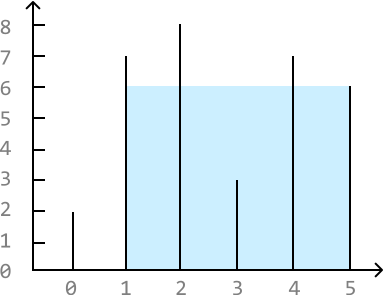
Input: heights = [2, 7, 8, 3, 7, 6]
Output: 24
Intuitsiya
Agar bizda ikkita vertikal chiziq, heights[i] va heights[j] bo'lsa, ular orasiga saqlanishi mumkin bo'lgan suv miqdori formula bilan hisoblanadi.
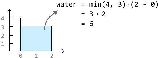
Boshqacha aytganda, idishning maydoni ikki narsaga bog'liq:
- To'g'ri to'rtburchakning kengligi.
- Ikki chiziqning qisqaroq biri bilan belgilanadigan to'g'ri to'rtburchakning balandligi.
Ushbu masalaga qo'pol kuch yechimi barcha chiziqlar juftlarini tekshirib, eng katta idishni qaytarishni o'z ichiga oladi.
from typing import List

def largest_container_brute_force(heights: List[int]) -> int:
   n = len(heights)
   max_water = 0
   # Find the maximum amount of water stored between all pairs of lines.
   for i in range(n):
       for j in range(i + 1, n):
           water = min(heights[i], heights[j]) * (j - i)
           max_water = max(max_water, water)
   return max_water
Barcha mumkin bo'lgan qiymatlar juftlarini qidirish O(n²) vaqt oladi, bu yerda n massiv uzunligini bildiradi.
Eng katta idishga ega bo'lish uchun ham balandlik, ham kenglik imkon qadar katta bo'lishini xohlaymiz.
Eng katta balandlikka ega idishni qanday topish darhol aniq emas, chunki chiziqlarning balandliklari turlichadir.
Shuning uchun, kenglikni maksimallashtirish uchun har bir massiv uchida ko'rsatkich o'rnatishdan boshlaymiz. Keyin eng katta idishni topish uchun ko'rsatkichlarni ichkariga siljita olamiz.
Ko'rsatkichni ichkariga siljitish — chap ko'rsatkichni o'ngga yoki o'ng ko'rsatkichni chapga ko'chirishni bildiradi.
Quyidagi misolni ko'rib chiqing:
![Image represents a bar chart visualizing the data contained within the Python list `heights = [2, 7, 8, 3, 7, 6]`. The horizontal axis represents the index of each element in the list (0 through 5), while the vertical axis represents the value of each element, ranging from 0 to 8. Each vertical bar corresponds to an element in the list; its height corresponds to the element's value. For example, the first bar at index 0 has a height of 2, the second bar at index 1 has a height of 7, and so on. The vertical axis is marked with numerical labels (0 through 8) indicating the height of the bars, and the horizontal axis is implicitly marked by the position of the bars, corresponding to the list indices. The arrowheads on the axes indicate the direction of increasing values.](https://bytebytego.com/images/courses/coding-patterns/two-pointers/largest-container/image-01-04-2-2GSU2V4T.svg?dpl=dpl_Gs7zfM6MUzjTBjcjps1LqXtb9QmD)
Eng keng idish 10 birlik suv saqlay oladi. Bu biz topgan eng katta idish bo'lgani uchun max_water ni 10 ga yangilaymiz.
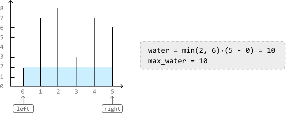
Qanday davom etish kerak? Ixtiyoriy ko'rsatkichni ichkariga siljitish qisqaroq kenglikka ega idishga olib keladi. Bu balandlikni aniqlovchi omil sifatida qoldiradi.
![Image represents a visual explanation of a coding pattern, likely related to algorithms operating on arrays or lists. The left side shows a bar chart with a horizontal axis labeled from 0 to 5 and a vertical axis representing height from 0 to 8. Several bars of varying heights are displayed; the heights are implicitly represented by the vertical extent of the bars. A light-blue rectangle fills the area below the height of the bars, representing a water level. An orange box labeled 'left' points to the leftmost bar, and another orange box labeled 'right' points to the rightmost bar. These labels 'left' and 'right' likely represent index pointers within an array. On the right side, a light-grey dashed-bordered box contains a conditional statement in code-like notation: `heights[left] < heights[right] → left += 1`. This indicates that if the height at the index `left` is less than the height at the index `right`, then the `left` index is incremented by 1. The arrow implies a flow of information or control; the condition's evaluation dictates the update of the `left` pointer. The overall diagram illustrates a step within an algorithm, possibly for finding the largest rectangular area in a histogram or a similar problem involving array traversal and comparison.](https://bytebytego.com/images/courses/coding-patterns/two-pointers/largest-container/image-01-04-4-HYLGZML2.svg?dpl=dpl_Gs7zfM6MUzjTBjcjps1LqXtb9QmD)
Joriy idish 24 birlik suv ushlab turishi mumkin — hozirgacha eng ko'p. Shuning uchun max_water ni yangilaymiz.
![Image represents a bar chart illustrating a coding pattern, likely related to finding the maximum area of water trapped between vertical bars. The horizontal axis shows indices (0 to 5), and the vertical axis represents heights. Vertical bars of varying heights are drawn at each index; their heights are 2, 6, 6, 3, 6, and 0 respectively. A light-blue area is filled between the bars at indices 1, 2, 3, and 4, representing the trapped water. Arrows labeled 'left' and 'right' point towards the x-axis, indicating the direction of traversal in an algorithm. A separate box contains code snippets: `water = min(7, 6) * (5 - 1) = 24` calculates the water trapped between specific bars (likely using the minimum height as the limiting factor and the distance between them), `max_water = 24` stores the maximum water found so far, and `heights[left] > heights[right] → right -= 1` shows a conditional statement, suggesting an algorithm iterates from left and right, moving the right pointer inwards if the left bar is taller. The overall diagram visually explains a two-pointer approach to solving a 'trapping rain water' problem.](https://bytebytego.com/images/courses/coding-patterns/two-pointers/largest-container/image-01-04-5-RVU2TMEL.svg?dpl=dpl_Gs7zfM6MUzjTBjcjps1LqXtb9QmD)
Bundan keyin, chap va o'ng chiziqlar balandligi teng bo'lgan holatga duch kelamiz. Bu holatda kenglik qisqaroq bo'ladi, balandlik esa hal qiluvchi omil bo'lib qoladi.
Ixtiyoriy ko'rsatkichni ichkariga siljitish qisqaroq kenglikka ega idishga olib keladi va balandlik hal qiluvchi omil bo'lib qoladi.
Shuning uchun, faqat bitta ko'rsatkich orqali balandlikni oshira olmaymiz, ikkala ko'rsatkichni ham ichkariga siljitamiz.
![Image represents a bar chart illustrating a 'two-pointer' approach to finding the maximum area that can be contained between vertical bars. The horizontal axis shows indices (0 to 5), and the vertical axis represents height. Several vertical bars of varying heights are depicted; one bar at index 0 has a height of 2, a group of bars from index 1 to 3 have a height of 7, and a bar at index 3 has a height of 6. The area between the bars at indices 1 and 3 is shaded light blue, representing the calculated water trapped between them. Two orange rectangular boxes labeled 'left' and 'right' point to the indices 1 and 4 respectively, indicating the pointers used in the algorithm. A separate box displays calculation details: `water = min(7, 7) * (4 - 1) = 21`, showing the calculation of the water trapped between the pointers; `max_water = 24` indicates the maximum water trapped found so far; and `heights[left] == heights[right] => left += 1 and right -= 1` describes the algorithm's logic: if the heights at the left and right pointers are equal, both pointers move inwards.](https://bytebytego.com/images/courses/coding-patterns/two-pointers/largest-container/image-01-04-6-POJJUDHN.svg?dpl=dpl_Gs7zfM6MUzjTBjcjps1LqXtb9QmD)
Endi, o'ng chiziq suv balandligini cheklayapti. Shuning uchun o'ng ko'rsatkichni ichkariga siljitamiz:
![Image represents a diagram illustrating a coding pattern, likely related to finding the maximum trapped rainwater between vertical bars. The left side shows a bar chart with vertical bars of varying heights (1, 7, 3, 7, 6) at positions 0, 1, 2, 3, 4, 5 respectively on the x-axis and heights on the y-axis. A light-blue rectangle is filled between bars of height 3 and 7 at positions 2 and 3, representing trapped water. Below the chart, orange rectangular boxes labeled 'left' and 'right' indicate pointers or indices used to iterate through the bars. An arrow points upwards from 'left' to the bar at position 2 and another from 'right' to the bar at position 3. The right side contains a light-grey box with code-like annotations. These annotations show a calculation: `water = min(8, 3) * (3 - 2) = 3`, indicating the calculation of water trapped between two bars; `max_water = 24`, representing the maximum trapped water; and `heights[left] > heights[right] => right -= 1`, suggesting a conditional statement controlling the movement of the 'right' pointer based on the heights of the bars at the 'left' and 'right' indices. The overall diagram visually explains an algorithm for calculating maximum trapped rainwater using two pointers.](https://bytebytego.com/images/courses/coding-patterns/two-pointers/largest-container/image-01-04-7-M2EWX37E.svg?dpl=dpl_Gs7zfM6MUzjTBjcjps1LqXtb9QmD)
Nihoyat, chap va o'ng ko'rsatkichlar uchrashtirdi. Qidiruvni shu yerda yakunlab max_water ni qaytaramiz:
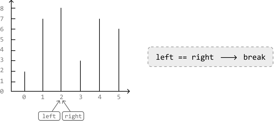
Misoldagi qarorlarga asoslanib, mantiqni xulosalaymiz:
- Agar chap chiziq kichikroq bo'lsa, chap ko'rsatkichni ichkariga siljiting.
- Agar o'ng chiziq kichikroq bo'lsa, o'ng ko'rsatkichni ichkariga siljiting.
- Agar ikkala chiziq ham bir xil balandlikda bo'lsa, ikkala ko'rsatkichni ham ichkariga siljiting.
Amalga oshirish
from typing import List

def largest_container(heights: List[int]) -> int:
    max_water = 0
    left, right = 0, len(heights) - 1
    while (left < right):
        # Calculate the water contained between the current pair of lines.
        water = min(heights[left], heights[right]) * (right - left)
        max_water = max(max_water, water)
        # Move the pointers inward, always moving the pointer at the shorter line. If
        # both lines have the same height, move both pointers inward.
        if (heights[left] < heights[right]):
            left += 1
        elif (heights[left] > heights[right]):
            right -= 1
        else:
            left += 1
            right -= 1
    return max_water
Murakkablik Tahlili
Vaqt murakkabligi: largest_container ning vaqt murakkabligi O(n), chunki eng yomon holatda ikki ko'rsatkich texnikasidan foydalanib taxminan n ta iteratsiya bajaramiz.
Xotira murakkabligi: Biz faqat doimiy sondagi o'zgaruvchilar ajratdik, shuning uchun xotira murakkabligi O(1).
Test Holatlari
Ushbu tushuntirish davomida muhokama qilingan misollarga qo'shimcha ravishda, quyida kodingizni sinash paytida ko'rib chiqiladigan boshqa misollar keltirilgan.
| Input | Expected output | Description |
|---|---|---|
heights = [] | 0 | Tests an empty array. |
heights = [1] | 0 | Tests an array with just one element. |
heights = [0, 1, 0] | 0 | Tests an array with no containers that can contain water. |
heights = [3, 3, 3, 3] | 9 | Tests an array where all heights are the same. |
heights = [1, 2, 3] | 2 | Tests an array with strictly increasing heights. |
heights = [3, 2, 1] | 2 | Tests an array with strictly decreasing heights. |
Nollarni Oxiriga Siljitish
Nollarni Oxiriga Siljitish
Butun sonlar massivi berilgan, nolsiz elementlarning nisbiy tartibini saqlab, barcha 0 larni massiv oxiriga ko'chiring. Bu o'z joyida amalga oshirilishi kerak.
Misol:
Input: nums = [0, 1, 0, 3, 2]
Output: [1, 3, 2, 0, 0]
Intuitsiya
Bu masalaning uchta asosiy talabi bor:
- Barcha nollarni massiv oxiriga ko'chiring.
- Nolsiz elementlarning nisbiy tartibini saqlang.
- O'zgartirishni o'z joyida amalga oshiring.
Bu masalaga sodda yondashuv — alohida massiv (temp) yordamida chiqishni qurishdir. Barcha nolsiz elementlarni temp ga, keyin esa nollarni qo'shishimiz mumkin.
Massivning chap tomonidagi nolsiz elementlarni avval aniqlab ko'chirish orqali ularning nisbiy tartibini saqlaymiz.
def shift_zeros_to_the_end_naive(nums: List[int]) -> None:
    temp = [0] * len(nums)
    i = 0
    # Add all non-zero elements to the left of 'temp'.
    for num in nums:
        if num != 0:
            temp[i] = num
            i += 1
    # Set 'nums' to 'temp'.
    for j in range(len(nums)):
        nums[j] = temp[j]
Afsuski, bu yechim kiritilgan massivni o'z joyida o'zgartirish — uchinchi talabni buzadi.
Biroq, bu yondashuvdan muhim tushuncha olish mumkin. Ayniqsa, nolsiz elementlarning massivning chap tomoniga joylashtirilishi kerakligiga e'tibor bering.
![The image represents a data transformation process. It shows an input array `[0 1 0 2 3]` enclosed in square brackets. A light-blue rectangular box highlights the non-zero elements (1, 2, and 3) within this array. A solid black arrow points from the input array to an output array `[1 2 3 0 0]`. Below the input array, the text 'non-zero numbers go here' in light-blue indicates that the transformation involves extracting only the non-zero numbers. Light-blue horizontal lines are drawn under both the input and output arrays, visually connecting the non-zero elements in the input to their corresponding positions in the output, implying a direct mapping of non-zero values. The zeros in the input array are preserved in the output array, maintaining the original array's length.](https://bytebytego.com/images/courses/coding-patterns/two-pointers/shift-zeros-to-the-end/image-01-05-1-IJRTSKQD.svg?dpl=dpl_Gs7zfM6MUzjTBjcjps1LqXtb9QmD)
Agar nolsiz elementlar joylashadigan massivning yuqoridagi diapazonini takrorlash imkoni bo'lsa, biz kiritilgan massivni o'z joyida o'zgartirishimiz mumkin edi.
Ikki ko'rsatkich Buning uchun ikki ko'rsatkichdan foydalanishimiz mumkin:
- Nolsiz elementlar joylashtirilishi kerak bo'lgan massivning chap qismini takrorlash uchun chap ko'rsatkich.
- Nolsiz elementlarni topish uchun o'ng ko'rsatkich.
Quyidagi misolni ko'rib chiqing. Chap va o'ng ko'rsatkichlarni massiv boshiga qo'yib boshlang.
![Image represents a visualization of a coding pattern, likely illustrating pointer manipulation within an array. The top section shows two gray boxes labeled 'left' and 'right' pointing downwards to an array `[0 1 0 2 3]`. This represents the initial state of the array and the pointers. Below, a second similar arrangement shows the array after a step in the algorithm. The 'left' pointer remains unchanged, but the 'right' pointer (shown in orange) has moved one position to the right. A dashed gray box in the middle displays a conditional statement: `nums[right] == 0 → right += 1`, indicating that if the element at the index pointed to by 'right' is equal to 0, then the value of 'right' is incremented. The dashed line connecting the 'right' pointer in the second array to the conditional statement visually connects the conditional check to the pointer's movement. The overall diagram illustrates a single iteration of an algorithm that likely involves traversing and manipulating an array using two pointers.](https://bytebytego.com/images/courses/coding-patterns/two-pointers/shift-zeros-to-the-end/image-01-05-2-NAB3RLLM.svg?dpl=dpl_Gs7zfM6MUzjTBjcjps1LqXtb9QmD)
Esda tuting, biz chap ko'rsatkichni faqat nolsiz elementlar joylashtirilishi kerak bo'lgan joyni kuzatish uchun ishlatamiz. Shuning uchun o'ng ko'rsatkich nolsiz elementni topmaguncha chap ko'rsatkichni siljitmaymiz.
Endi o'ng ko'rsatkichdagi qiymat nolsiz. Keling, bu holatni qanday boshqarishni muhokama qilaylik.
1. Chap va o'ngdagi elementlarni almashtirish: Avval o'ng ko'rsatkichdagi elementni chap ko'rsatkich ko'rsatgan pozitsiyaga ko'chirishni xohlaymiz.
![Image represents a visual depiction of a sorting algorithm's step. Two rectangular boxes labeled 'left' and 'right' are positioned above a horizontal array `[0 1 0 2 3]`. Arrows descend from 'left' and 'right' pointing to the array elements at indices 0 and 1 respectively. A dashed-line rectangle to the right contains the conditional statement 'nums[right] != 0 → swap(nums[left], nums[right])', indicating that if the element at the index pointed to by 'right' (which is 1 in this case) is not equal to 0, then a swap operation occurs between the elements at the indices pointed to by 'left' and 'right'. The 'nums' refers to the array, and 'left' and 'right' act as index pointers. The arrow '→' signifies the conditional execution of the swap function.](https://bytebytego.com/images/courses/coding-patterns/two-pointers/shift-zeros-to-the-end/image-01-05-3-NHRSBRLL.svg?dpl=dpl_Gs7zfM6MUzjTBjcjps1LqXtb9QmD)
![Image represents a visual depiction of a swap operation within a sorting algorithm, likely a variation of quicksort or similar. At the top, two rectangular boxes labeled 'left' and 'right' are shown, each with a downward-pointing arrow. These arrows point to a numerical array represented as `[1 0 2 3]`, where the numbers 1 and 0 are highlighted in light peach circles. A gray horizontal line connects the numbers 1 and 0, indicating their positions within the array. A curved orange arrow, labeled 'swapped,' arcs underneath the line, connecting the circled 1 and 0, illustrating the exchange of these two elements. The overall diagram demonstrates a single swap step in a sorting process, where the values pointed to by 'left' and 'right' pointers are interchanged.](https://bytebytego.com/images/courses/coding-patterns/two-pointers/shift-zeros-to-the-end/image-01-05-4-5ODTEVDH.svg?dpl=dpl_Gs7zfM6MUzjTBjcjps1LqXtb9QmD)
2. Ko'rsatkichlarni oshirish:
- Almashtirish tugagach, chap ko'rsatkichni keyingi nolsiz element joylashishi kerak bo'lgan pozitsiyaga o'rnatish uchun oshirishimiz kerak.
- Keyingi nolsiz elementni qidirish uchun o'ng ko'rsatkichni ham oshiraylik.
![The image represents a simple illustration of a coding pattern, possibly related to array manipulation or pointer movement. Two rectangular boxes labeled 'left' and 'right' are positioned above a horizontal line segment. Downward arrows connect each box to a number below the line. The numbers below the line are arranged as an array-like structure: `[1 0 0 2 3]`. A dashed-line rectangle to the right contains the text 'left += 1, right += 1', indicating an operation where the values associated with 'left' and 'right' are incremented by 1. The arrows suggest that the 'left' and 'right' variables might represent indices or pointers into the array, and the operation in the dashed box describes how these indices are updated. The overall diagram visually depicts a step in an algorithm that involves iterating or manipulating an array using two pointers.](https://bytebytego.com/images/courses/coding-patterns/two-pointers/shift-zeros-to-the-end/image-01-05-5-IAQXF357.svg?dpl=dpl_Gs7zfM6MUzjTBjcjps1LqXtb9QmD)
![Image represents a diagram illustrating a coding pattern, possibly related to array traversal or pointer manipulation. Two rectangular boxes labeled 'left' (in orange) and 'right' (in gray) are positioned at the top. A solid downward-pointing arrow extends from each box, indicating data flow. These arrows point to the numbers 0 and 0 respectively, which are situated below on a horizontal gray line representing an array or sequence. The number 1 is placed to the left of the 0 from the 'left' box, and the number 2 and 3 are placed to the right of the 0 from the 'right' box, all on the same horizontal line, enclosed within square brackets `[ ]` to denote an array structure. A dashed orange arrow connects the 'left' box's output (0) to the number 1, suggesting a possible indirect or conditional relationship or data flow. The overall arrangement suggests a process where the 'left' and 'right' elements might represent pointers or indices that traverse the array, potentially converging or interacting at a central point (the 0s).](https://bytebytego.com/images/courses/coding-patterns/two-pointers/shift-zeros-to-the-end/image-01-05-6-VEUCCWPT.svg?dpl=dpl_Gs7zfM6MUzjTBjcjps1LqXtb9QmD)
Bu mantiqni massivning qolgan qismiga qo'llab, har bir bosqichda keyingi nolsiz elementni topish uchun o'ng ko'rsatkichni oshirib boramiz.
![Image represents a diagram illustrating a coding pattern, possibly within a sorting or searching algorithm. Two rectangular boxes labeled 'left' and 'right' are positioned above a horizontal array represented by `[1 0 0 2 3]`. Arrows descend from 'left' and 'right' pointing to the array elements at indices 1 and 2 respectively (the values 0 and 0). A separate, light-grey, dashed-bordered rectangle to the right contains a conditional statement: `nums[right] == 0 -> right += 1`. This indicates that if the element at the index `right` in the `nums` array is equal to 0, then the value of `right` is incremented by 1. The diagram visually shows the variables `left` and `right` potentially used as pointers or indices within the array, and the conditional statement describes a step in an algorithm that modifies the `right` pointer based on the value of the array element it points to.](https://bytebytego.com/images/courses/coding-patterns/two-pointers/shift-zeros-to-the-end/image-01-05-7-AFMMQFWI.svg?dpl=dpl_Gs7zfM6MUzjTBjcjps1LqXtb9QmD)
![Image represents a simplified illustration of a data structure, possibly an array, being manipulated. Two rectangular boxes, labeled 'left' (in gray) and 'right' (in orange), represent pointers or indices. A gray horizontal line depicts an array containing the elements [1, 0, 0, 2, 3]. A solid downward-pointing arrow from 'left' points to the element '0' at index 1, indicating that the 'left' pointer is currently at this position. An orange downward-pointing arrow from 'right' points to the element '2' at index 3, showing the 'right' pointer's position. A dashed orange curved arrow connects the 'right' pointer to the element '0' at index 2, suggesting a potential movement or operation involving this element. The overall arrangement visualizes the pointers' positions within the array and hints at a possible algorithm or process involving these pointers, perhaps related to partitioning or searching within the data structure.](https://bytebytego.com/images/courses/coding-patterns/two-pointers/shift-zeros-to-the-end/image-01-05-8-EIRQV4PD.svg?dpl=dpl_Gs7zfM6MUzjTBjcjps1LqXtb9QmD)
![Image represents a visual depiction of a step in a sorting algorithm, likely a comparison-based sort. Two rectangular boxes labeled 'left' and 'right' are positioned above a horizontal array `[1, 0, 0, 2, 3]`. Arrows descend from 'left' and 'right' pointing to the array elements at indices 1 and 4 respectively (0 and 2). A dashed-line rectangle to the right displays the condition `nums[right] != 0` followed by a right arrow and the action `swap(nums[left], nums[right])`. This indicates that if the element at the index pointed to by 'right' (which is 2) is not equal to 0, then the elements at the indices pointed to by 'left' and 'right' (0 and 2) will be swapped. The diagram illustrates a single comparison and potential swap operation within a larger sorting process.](https://bytebytego.com/images/courses/coding-patterns/two-pointers/shift-zeros-to-the-end/image-01-05-9-M2BOBUFL.svg?dpl=dpl_Gs7zfM6MUzjTBjcjps1LqXtb9QmD)
![Image represents a visual depiction of a swapping operation within an array. The diagram shows an array `[1, 2, 0, 3]` with two pointers, labeled 'left' and 'right,' initially pointing to the elements 2 and 0 respectively. Arrows from rectangular boxes labeled 'left' and 'right' indicate the pointers' positions. A gray horizontal line connects the elements 1, 2, 0, and 3, representing the array. A curved orange arrow labeled 'swapped' shows the exchange of the values at the 'left' and 'right' pointer positions. To the right, a light gray, dashed-bordered rectangle contains the operation `left += 1, right += 1`, indicating that after the swap, both pointers will increment their positions by one in the next iteration. The overall image illustrates a single step in a sorting algorithm, likely involving a swap and pointer movement.](https://bytebytego.com/images/courses/coding-patterns/two-pointers/shift-zeros-to-the-end/image-01-05-10-67EQWWFS.svg?dpl=dpl_Gs7zfM6MUzjTBjcjps1LqXtb9QmD)
![Image represents a diagram illustrating a simple coding pattern, possibly related to array manipulation or pointer movement. The diagram shows a numerical array `[1 2 0 0 3]` represented horizontally. Above the array, two rectangular boxes labeled 'left' and 'right' in orange are positioned. A solid orange arrow descends from 'left' pointing to the element '0' in the second position from the left within the array. Similarly, a solid orange arrow descends from 'right' pointing to the element '3' at the right end of the array. Dashed orange lines curve from 'left' to the element '2' and from 'right' to the element '0' in the third position, suggesting a potential search or traversal pattern. The overall arrangement suggests a process where two pointers, one starting from the left and the other from the right, might be moving towards the center of the array, potentially for comparison, searching, or merging operations.](https://bytebytego.com/images/courses/coding-patterns/two-pointers/shift-zeros-to-the-end/image-01-05-11-F5CI56AA.svg?dpl=dpl_Gs7zfM6MUzjTBjcjps1LqXtb9QmD)
![Image represents a visual depiction of a step in a sorting algorithm, likely a part of a larger process. Two rectangular boxes labeled 'left' and 'right' are positioned above a numerical array `[1, 2, 0, 0, 3]`. Arrows descend from 'left' and 'right' pointing to the '0' elements within the array, indicating these are the current indices being considered. A dashed-line rectangle to the right shows a conditional statement: `nums[right] != 0 → swap(nums[left], nums[right])`. This indicates that if the element at the index 'right' is not equal to 0, then a `swap` function is called to exchange the values at the 'left' and 'right' indices within the `nums` array. The arrow represents the flow of control based on the condition.](https://bytebytego.com/images/courses/coding-patterns/two-pointers/shift-zeros-to-the-end/image-01-05-12-XNRYRK65.svg?dpl=dpl_Gs7zfM6MUzjTBjcjps1LqXtb9QmD)
![Image represents a visual depiction of a swapping operation within an array. The diagram shows an array `[1, 2, 3, 0]` with two pointers, 'left' and 'right', initially pointing to the elements 3 and 0 respectively. Rectangular boxes labeled 'left' and 'right' above indicate the pointers' origins. A downward-pointing arrow from each box connects to its corresponding element in the array. The elements 3 and 0 are highlighted in light peach. A gray horizontal line connects the elements 1 and 2, visually representing the array's structure. A curved orange arrow labeled 'swapped' connects the highlighted elements 3 and 0, indicating that these elements have been exchanged. To the right, a light gray, dashed-bordered rectangle displays the operation performed: `→ left += 1, right += 1`, signifying that after the swap, both pointers will increment their positions by one.](https://bytebytego.com/images/courses/coding-patterns/two-pointers/shift-zeros-to-the-end/image-01-05-13-EFX6N3MT.svg?dpl=dpl_Gs7zfM6MUzjTBjcjps1LqXtb9QmD)
![Image represents a diagram illustrating a coding pattern, possibly related to array manipulation or pointer movement. The diagram shows a light-blue rectangular array `[1 2 3]` with a light-blue underline indicating its boundaries. Two orange rectangular boxes labeled 'left' and 'right' are positioned above the array. Dashed orange arrows point downwards from 'left' and 'right' to the array elements. The 'left' arrow points to the first element (1) and the 'right' arrow points to the last element (3). The arrows suggest that the 'left' and 'right' variables might represent pointers or indices that can be manipulated to traverse the array. The empty space `∅` between the array and the pointers suggests an initial state or a potential intermediate step in an algorithm. The overall structure suggests a two-pointer approach commonly used in algorithms like merging or partitioning.](https://bytebytego.com/images/courses/coding-patterns/two-pointers/shift-zeros-to-the-end/image-01-05-14-RQIWELLT.svg?dpl=dpl_Gs7zfM6MUzjTBjcjps1LqXtb9QmD)
Barcha almashtirishlar tugagach, barcha nollar mo'ljallangan tarzda massivning o'ng tomoniga joylashadi, nolsiz elementlarning nisbiy tartibi esa saqlanadi.
Amalga oshirish
O'ng ko'rsatkich nolni ko'rsatadimi yoki ko'rsatmadimi, har doim oldinga siljitishimiz e'tiboringizni tortgan bo'lishi mumkin.
def shift_zeros_to_the_end(nums: List[int]) -> None:
    # The 'left' pointer is used to position non-zero elements.
    left = 0
    # Iterate through the array using a 'right' pointer to locate non-zero
    # elements.
    for right in range(len(nums)):
        if nums[right] != 0:
            if right != left:
                nums[left], nums[right] = nums[right], nums[left]
            # Increment 'left' since it now points to a position already occupied
            # by a non-zero element.
            left += 1
Murakkablik Tahlili
Vaqt murakkabligi: shift_zeros_to_the_end ning vaqt murakkabligi O(n), bu yerda n massiv uzunligini bildiradi.
Xotira murakkabligi: Siljitish o'z joyida amalga oshirilganligi sababli xotira murakkabligi O(1).
Test Holatlari Muhokama qilingan misollarga qo'shimcha ravishda, quyida kodingizni sinash paytida ko'rib chiqiladigan ko'proq misollar keltirilgan.
| Input | Expected output | Description |
|---|---|---|
nums = [] | [] | Tests an empty array. |
nums = [0] | [0] | Tests an array with one 0. |
nums = [1] | [1] | Tests an array with one 1. |
nums = [0, 0, 0] | [0, 0, 0] | Tests an array with all 0s. |
nums = [1, 3, 2] | [1, 3, 2] | Tests an array with all non-zeros. |
nums = [1, 1, 1, 0, 0] | [1, 1, 1, 0, 0] | Tests an array with all zeros already at the end. |
nums = [0, 0, 1, 1, 1] | [1, 1, 1, 0, 0] | Tests an array with all zeros at the start. |
Keyingi Leksikografik Ketma-ketlik
Keyingi Leksikografik Ketma-ketlik
Kichik harfli ingliz harflaridan iborat satr berilgan, keyingi leksikografik ketma-ketlikni ifodalovchi yangi satrni hosil qilish uchun belgilarni qayta tartiblang. Agar satr eng oxirgi leksikografik ketma-ketlik bo'lsa, birinchi ketma-ketlikni qaytaring (ya'ni satrni o'sish tartibida tartiblang).
Misol 1:
Input: s = 'abcd'
Output: 'abdc'
Tushuntirish: "abdc" — "abcd" ni qayta tartiblaganidan keyin leksikografik tartibdagi keyingi ketma-ketlik.
Misol 2:
Input: s = 'dcba'
Output: 'abcd'
Tushuntirish: "dcba" leksikografik tartibdagi oxirgi ketma-ketlik bo'lganligi sababli, birinchi ketma-ketlikni qaytaramiz.
Cheklovlar:
- Satr kamida bitta belgi o'z ichiga oladi.
Intuitsiya
Yechim ishlab chiqishdan oldin, keyingi leksikografik ketma-ketlik nima ekanligini to'g'ri tushunganligimizni tekshiraylik.
Muhim tafsilot shundan iboratki, satrning keyingi leksikografik ketma-ketligi joriy satrdan leksikografik jihatdan kattaroqdir.
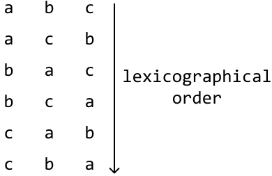
Har bir harfni uning raqamli ekvivalentiga o'tkazganimizda ketma-ketlikdagi satrlarning o'sib borish tartibini ko'rishimiz mumkin.
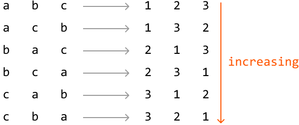
Bundan tashqari, "abc" dan keyingi ketma-ketlik "acb" ekanligini ko'ramiz, bu "abc" dan boshlanadiganlarning birinchi ketma-ketligidir.
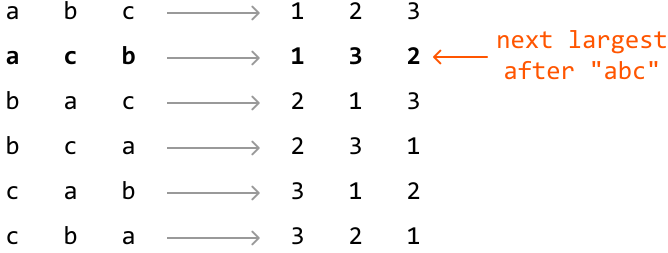
Bu bizga nima topishimiz kerakligiga doir ma'lumot beradi. Keyingi leksikografik satr:
- Asl satrdan eng kichik mumkin bo'lgan leksikografik oshishni amalga oshiradi.
- Asl satr bilan bir xil harflardan foydalanadi.
Qaysi belgilarni qayta tartiblash kerakligini aniqlash Maqsadimiz eng kichik mumkin bo'lgan oshishni amalga oshirish bo'lganligi sababli, satrning o'ng tomonidagi belgilarni qayta tartiblaymiz.
Nima uchunligini tushunish uchun satrning qiymatini "oshirishni" tasavvur qiling. Eng o'ng tarafdagi harfni oshirish minimal oshishga olib keladi.
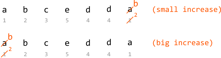
Shuning uchun, iloji bo'lsa satrning o'ng tomonidagi belgilarni qayta tartiblaymiz.
Muhim tushuncha shundan iboratki, leksikografik ketma-ketlikdagi oxirgi satr (ya'ni eng katta permutatsiya) o'smaydigan tartibda joylashtirilgan.

Bu bizga qanday yordam beradi? Biz satrning o'ng tomonidagi belgilarni qayta tartiblaymiz, lekin qanchasini qayta tartiblaymiz? Javob: eng qisqa suffiksni, ya'ni leksikografik jihatdan o'smaydigan eng uzun o'ng suffiksni.
Misol sifatida "abcedda" satrini olaylik. Biz undan o'ngdan chapga o'smaydigan ketma-ketlikni buzadigan birinchi belgi — "pivot" ni topish maqsadida aylanamiz.
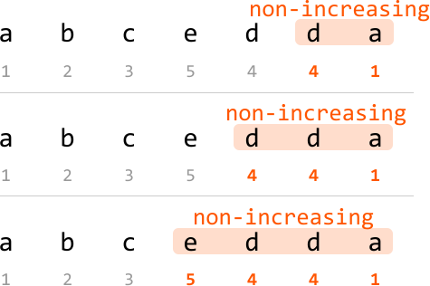
Biroq, keyingi 'c' belgisi o'smaydigan ketma-ketlikni buzadi:

Keling, ushbu belgini pivot deb ataymiz:
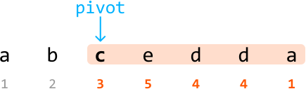
Agar pivot topilmasa, satr allaqachon oxirgi leksikografik ketma-ketlik ekanligini bildiradi. Bu holda birinchi ketma-ketlikni qaytaramiz — satrni o'sish tartibida tartiblash.

Belgilarni qayta tartiblash Qayta tartiblanishi kerak bo'lgan eng qisqa suffiksni aniqlaganidan so'ng, keyingi maqsad pivot pozitsiyasidagi belgini oshirishdir.
Pivot pozitsiyasidagi belgini kattalashtirish uchun pivotni kattaroq belgi bilan almashtirishimiz kerak.
Misolimizda pivot ('c') qaysi belgi bilan almashtirilishi kerak? Biz uni pivotdan kattaroq, lekin imkon qadar kichik bo'lgan belgi bilan almashtirishni xohlaymiz.
Pivot dan keyingi quyi satr leksikografik jihatdan o'smaydigan bo'lganligi sababli, eng o'ng tarafdagi vorissni (pivotdan kattaroq eng o'ng belgi) ikkilik qidiruv yordamida topa olamiz.
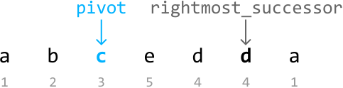
Endi pivotni eng o'ng tarafdagi voris bilan almashtiramiz:

Pivot pozitsiyasidagi belgi oshirildi, shuning uchun keyingi permutatsiyani olish uchun pivotdan keyingi quyi satrni minimallashtirish kerak.
Muhim kuzatuv shundan iboratki, oldingi almashtirishdan keyin pivotdan keyingi quyi satr hali ham leksikografik jihatdan o'smaydigan.

Bu shuni anglatadiki, ushbu quyi satrning permutatsiyasini uni teskari aylantirish orqali minimallashtirishimiz mumkin:

Mana shunday, keyingi leksikografik ketma-ketlikni topdik! Bu masalada ishlatiladigan ikki ko'rsatkich strategiyasi bosqichli aylanish namunasiga mos keladi.
Keyingi leksikografik ketma-ketlikni aniqlashda ko'plab qadamlar mavjud. Shuning uchun qisqacha xulosa:
- Pivotni toping.
- Pivot — satrning o'ng tomonidan o'smaydigan ketma-ketlikni buzadigan birinchi belgidir.
- Agar pivot topilmasa, satr allaqachon oxirgi leksikografik ketma-ketlikda va natija birinchi ketma-ketlikdir.
- Pivotning eng o'ng tarafdagi vorisini toping.
- Suffiksning leksikografik tartibini oshirish uchun eng o'ng tarafdagi vorissni pivot bilan almashtiring.
- Permutatsiyasini minimallashtirish uchun pivotdan keyingi suffiksni teskari aylantiring.
Amalga oshirish
def next_lexicographical_sequence(s: str) -> str:
    letters = list(s)
    # Locate the pivot, which is the first character from the right that breaks
    # non-increasing order. Start searching from the second-to-last position.
    pivot = len(letters) - 2
    while pivot >= 0 and letters[pivot] >= letters[pivot + 1]:
        pivot -= 1
    # If pivot is not found, the string is already in its largest permutation. In
    # this case, reverse the string to obtain the smallest permutation.
    if pivot == -1:
        return ''.join(reversed(letters))
    # Find the rightmost successor to the pivot.
    rightmost_successor = len(letters) - 1
    while letters[rightmost_successor] <= letters[pivot]:
        rightmost_successor -= 1
    # Swap the rightmost successor with the pivot to increase the lexicographical
    # order of the suffix.
    letters[pivot], letters[rightmost_successor] = (letters[rightmost_successor], letters[pivot])
    # Reverse the suffix after the pivot to minimize its permutation.
    letters[pivot + 1:] = reversed(letters[pivot + 1:])
    return ''.join(letters)
Murakkablik Tahlili
Vaqt murakkabligi: next_lexicographical_sequence ning vaqt murakkabligi O(n), bu yerda n satr uzunligini bildiradi.
Xotira murakkabligi: xotira murakkabligi O(n), chunki harflar ro'yxati uchun joy sarflanadi.
Test Holatlari
Muhokama qilingan misollarga qo'shimcha ravishda, quyida kodingizni sinash paytida ko'rib chiqiladigan ko'proq misollar keltirilgan.
| Input | Expected output | Description |
|---|---|---|
| s = 'a' | 'a' | Tests a string with a single character. |
| s = 'aaaa' | 'aaaa' | Tests a string with a repeated character. |
| s = 'ynitsed' | 'ynsdeit' | Tests a string with a random pivot character. |
Intervyu Maslahat
Maslahat: Tilni aniq ishlating. Intervyu davomida so'z tanlovida aniq bo'lish juda muhim.
Hash Xaritalar va To'plamlar
Hash Xaritalar va To'plamlarga Kirish
Hash Xaritalar va To'plamlarga Kirish
Intuitsiya
O'zingizni oziq-ovqat do'konida ishlab turgandek tasavvur qiling. Mijoz meva narxini so'radi. Agar sizda barcha mevalar ro'yxati bo'lsa, to'g'ri narxni topish uchun ro'yxatni boshidan oxirigacha ko'rib chiqishingiz kerak bo'ladi. Ammo agar siz narxlarni yodlab olgan bo'lsangiz, narxga darhol javob bera olasiz.
Hash xaritalar Hash xarita — tilga qarab hash jadval yoki lug'at deb ham ataladigan — kalit-qiymat juftlarini bog'laydigan ma'lumotlar strukturasi.
Meva narxlarini yodda saqlash — hash xaritalari yordamida meva narxlarini darhol qidirish imkoniyatiga kontseptual jihatdan o'xshaydi.
Hash xaritalar qidirish, kiritish va o'chirish uchun juda samarali, chunki ular odatda bu operatsiyalarni O(1) o'rtacha vaqt murakkabligi bilan bajaradi.
Hash xaritalarning xususiyatlari:
- Ma'lumotlar kalit-qiymat juftlari shaklida saqlanadi.
- Hash xaritalar takrorlarni saqlamaydi. Har bir kalit noyob bo'lib, har bir qiymatni aniq identifikatsiya qilish imkonini beradi.
- Hash xaritalar tartibsiz ma'lumotlar strukturasi, ya'ni kalitlar ma'lum tartibda saqlanmaydi.
Vaqt murakkabligi tahlili Quyida n hash xaritasidagi yozuvlar sonini bildiradi.
| Operation | Average case | Worst case | Description |
|---|---|---|---|
| Insert | Add a key-value pair to the hash map. | ||
| Access | Find or retrieve an element. | ||
| Delete | Delete a key-value pair. |
Kodlash intervyularida biz odatda hash xarita operatsiyalarini tez o'rtacha vaqt murakkabligi O(1) ga ega deb hisoblaymiz.
Hash to'plamlar Hash to'plamlar hash xaritalarning soddaroq shakli. Kalit-qiymat juftlarini saqlash o'rniga, ular faqat kalitlarni saqlaydi. Hash to'plamdan foydalanib, biz elementning to'plamda mavjudligini tezda tekshira olamiz.
Hash xaritalar yoki to'plamlardan qachon foydalanish kerak Hash xaritalarning keng tarqalgan qo'llanilishlariga lug'atlarni amalga oshirish, chastotalarni hisoblash, qiymatlarni indekslash kiradi.
Hash to'plamlarning keng tarqalgan qo'llanilishlariga noyob elementlarni saqlash, elementlarni ishlatilgan yoki tashrif buyurilgan deb belgilash va takrorlarni tekshirish kiradi.
Masala ta'rifida 'chastota', 'noyob', 'xarita', 'lug'at' yoki 'tez qidirish' kabi kalit so'zlarga e'tibor bering.
Hash xaritalar va to'plamlarni o'zlashtirish uchun muhim tushunchalar Bu bob hash xaritalar va to'plamlarning amaliy qo'llanilishini muhokama qiladi. Chuqurroq tushunish uchun quyidagilarni o'rganishni tavsiya qilamiz:
- Hash funksiyalar: kalitlarning hash jadvalidagi ma'lum qiymatlarga qanday moslanishining nozikliklarini o'rganing [1].
- To'qnashuv va to'qnashuv-boshqaruv texnikalar: hash to'qnashuvlarini hal qilish uchun zanjirlash yoki ochiq manzurlash kabi usullarni tushunish [2].
- Yuklama koeffitsientlari va qayta xashlash: bu hash jadvallarning qanday o'sishi va o'lchamini o'zgartirishi haqida tushunishni osonlashtiradi [3].
Hayotiy Misol
Veb-brauzer keshi: Hash xaritalar va to'plamlar real tizimlarning hamma joyida qo'llaniladi. Hash xaritalarning real hayotdagi klassik namunasi veb-brauzer keshidir.
Bob Mazmuni
Bu bob hash xaritalar va to'plamlarning eng mashhur qo'llanilishlarini o'z ichiga olgan masalalarni o'z ichiga oladi.
Juft Yig'indi - Tartiblangan Emas
Juft Yig'indi - Tartiblangan Emas
Butun sonlar massivi berilgan, maqsadga teng yig'indili ixtiyoriy ikkita sonning indekslarini qaytaring. Natijedagi indekslar tartibi muhim emas. Yechim topilishi kafolatlanadi.
Misol:
Input: nums = [-1, 3, 4, 2], target = 3
Output: [0, 2]
Tushuntirish: nums[0] + nums[2] = -1 + 4 = 3
Cheklovlar:
- Natijeida bir indeks ikki marta ishlatilishi mumkin emas.
Intuitsiya
Qo'pol kuch yendi massivdagi har bir mumkin bo'lgan juftni ko'rib chiqib ularning yig'indisi maqsadga teng ekanligini tekshirishdir.
To'ldiruvchi Biz (x, y) juftini topishimiz kerak, ya'ni x + y == target. Bu tenglamada ikki noma'lum mavjud: x va y. Agar x ni bilsak, y = target - x orqali y ni topa olamiz. y ga to'ldiruvchi deyiladi.
nums dagi har bir x son uchun x + y = target bo'ladigan boshqa y sonni topishimiz kerak, boshqacha aytganda, y = target - x.
Esda tuting, biz juftning o'zi emas, balki sonlar juftining indekslarini qaytarishimiz kerak. Shuning uchun ixtiyoriy sonning to'ldiruvchisi va unga mos indeksini topish usulimiz bo'lishi kerak.
Buni amalga oshirishning bir usuli — massiv bo'ylab aylanib har bir sonning to'ldiruvchisi va mos indeksini topishdir. Lekin bu O(n²) vaqt oladi.
Hash xarita Hash xarita juda zo'r ishlaydi, chunki biz qiymatlarni O(1) vaqtda saqlashimiz va qidirishimiz mumkin. Har bir son va uning indeksi hash xaritada kalit-qiymat juftlari sifatida saqlanadi.
![Image represents a transformation of a numerical array into a hashmap. The input is an array `[-1, 3, 4, 2]` with indices `[0, 1, 2, 3]` displayed beneath each element. A rightward arrow indicates the transformation process. The output is a hashmap labeled 'hashmap' which is represented as a table with two columns: 'num' and 'index'. The 'num' column lists the numbers from the input array: -1, 3, 4, and 2. The corresponding 'index' column shows the original index of each number in the input array: 0, 1, 2, and 3 respectively. The diagram illustrates how the original array's elements and their indices are reorganized into a key-value pair structure within the hashmap, where the number acts as the key and its original index acts as the value.](https://bytebytego.com/images/courses/coding-patterns/hash-maps-and-sets/pair-sum-unsorted/image-02-01-1-A3GUI4CR.svg?dpl=dpl_Gs7zfM6MUzjTBjcjps1LqXtb9QmD)
Bu ixtiyoriy sonning to'ldiruvchisi indeksini samarali qidirishga imkon beradi. Takroriy sonlar alohida ko'rib chiqilmasa ham bo'ladi, chunki bizga faqat bitta juft kerak.
Hash xaritani qo'llashning eng intuitiv usuli:
- Birinchi o'tishda hash xaritani har bir son va unga mos indeks bilan to'ldirish.
- Ikkinchi o'tishda har bir sonning to'ldiruvchisi hash xaritada mavjudligini tekshirish. Agar mavjud bo'lsa, juftning indekslarini qaytarish.
Quyida bu ikki o'tishli yondashuvning kod parchasi keltirilgan:
from typing import List

def pair_sum_unsorted_two_pass(nums: List[int], target: int) -> List[int]:
    num_map = {}
    # First pass: Populate the hash map with each number and its index.
    for i, num in enumerate(nums):
        num_map[num] = i
    # Second pass: Check for each number's complement in the hash map.
    for i, num in enumerate(nums):
        complement = target - num
        if complement in num_map and num_map[complement] != i:
            return [i, num_map[complement]]
    return []
Bu algoritm ikkita o'tishni talab qiladi. Buni faqat bittada amalga oshirish mumkinmi? Bir o'tishli yechim hash xaritani to'ldirish va to'ldiruvchini bir vaqtda tekshirishni anglatadi.
![Image represents a sample input for a search algorithm, likely a target-sum problem. The input consists of a numerical array [-1, 3, 4, 2] enclosed in square brackets, with each element implicitly indexed from 0 to 3 shown in grey below the array. This array is separated by a comma from the target value, which is explicitly stated as 'target = 3'. The arrangement suggests the algorithm's task is to find a subset of numbers within the array that sums up to the target value of 3. There is no explicit flow of information depicted; the image simply presents the input data for the algorithm to process.](https://bytebytego.com/images/courses/coding-patterns/hash-maps-and-sets/pair-sum-unsorted/image-02-01-2-ZQKF7AKS.svg?dpl=dpl_Gs7zfM6MUzjTBjcjps1LqXtb9QmD)
0-indeksdan boshlaymiz. Uning to'ldiruvchisi 3 - (-1) = 4 bo'ladi. Hash xaritamizda 4 bormi? Yo'q, hozir bo'sh. Shuning uchun -1 ni uning indeksi bilan birga hash xaritaga qo'shamiz.
![Image represents a data flow diagram illustrating a step in a coding pattern, likely involving hashmaps. An input array `[-1, 3, 4, 2]` with indices [0, 1, 2, 3] is shown. An orange arrow labeled 'x' points to the first element, -1. This array flows into a rectangular box labeled 'hashmap' with internal labels 'num' and 'index' suggesting it stores key-value pairs. To the right of the hashmap is a dashed-line box detailing the processing steps: first, it checks if the hashmap contains -1 (it doesn't); second, it calculates the complement of 4 (presumably within the context of the algorithm); and third, it adds the key-value pair (-1, 0) to the hashmap. The diagram visually depicts the input array, its processing through a hashmap, and the specific operations performed on the hashmap based on the input.](https://bytebytego.com/images/courses/coding-patterns/hash-maps-and-sets/pair-sum-unsorted/image-02-01-3-3EFCX52X.svg?dpl=dpl_Gs7zfM6MUzjTBjcjps1LqXtb9QmD)
Keyingi, 1-indeksga qaraylik. Uning to'ldiruvchisi (0) hash xaritada mavjud emas. Shuning uchun 3 va uning indeksini hash xaritaga qo'shamiz.
![Image represents a step-by-step illustration of a coding pattern involving a hashmap. An input array `[-1, 3, 4, 2]` is shown, with a small orange arrow pointing downwards to the element '3' at index 1, indicating the current element being processed. This array is then processed, resulting in a hashmap represented as a table with two columns labeled 'num' and 'index'. Currently, the hashmap contains only one entry: -1 at index 0. To the right of the hashmap is a dashed-line box containing three bullet points describing the processing logic: '- hashmap doesn't contain 3's', indicating that the current element (3) is not yet in the hashmap; 'complement (0)', suggesting a calculation of the complement (likely 0 in this context); and '- add (3, 1) to hashmap', indicating that the pair (3, 1) – the element and its index – will be added to the hashmap as the next step. The arrow between the array and the hashmap shows the data flow from the input array to the hashmap during processing.](https://bytebytego.com/images/courses/coding-patterns/hash-maps-and-sets/pair-sum-unsorted/image-02-01-4-DZH76J2A.svg?dpl=dpl_Gs7zfM6MUzjTBjcjps1LqXtb9QmD)
2-indeksda 4 ning to'ldiruvchisi (-1) hash xaritada mavjudligini ko'ramiz. Bu maqsadga yig'indili juft topilganligini bildiradi:
![Image represents a data transformation process. An input array `[-1, 3, 4, 2]` with indices [0, 1, 2, 3] is shown. A downward-pointing orange arrow labeled 'x' highlights the element '4' at index 2. This array is then transformed into a hashmap labeled 'hashmap' which has two key-value pairs. The key 'num' stores the number -1, and its corresponding value under the 'index' key is 3. The second key-value pair has 'num' as 0 and 'index' as 1. A separate dashed-line box describes the hashmap's content, stating that it 'contains 4's complement (-1)'. The arrow indicates the input array is processed to generate the hashmap, implying a mapping or counting operation where the complement of a number (in this case, 4's complement -1) and its index are stored.](https://bytebytego.com/images/courses/coding-patterns/hash-maps-and-sets/pair-sum-unsorted/image-02-01-5-LVD6664V.svg?dpl=dpl_Gs7zfM6MUzjTBjcjps1LqXtb9QmD)
Endi ikkala qiymat indekslarini qaytarishimiz mumkin. Kiritilgan massivdan 4 ning indeksini va hash xaritadan uning to'ldiruvchisining indeksini olamiz.
![Image represents a visual depiction of a coding pattern, likely for finding pairs in an array that sum to a target value (here, implicitly zero). The input is an array `[-1, 3, 4, 2]` with indices `0, 1, 2, 3` respectively, shown above a downward-pointing orange arrow labeled 'x', suggesting a target value or operation. This array is processed, with the element '4' (at index 2) highlighted in light green. A rightward arrow indicates the transformation of this array into a hashmap. The hashmap is represented as a box divided into two columns labeled 'num' and 'index'. The 'num' column contains the unique numbers from the input array (-1 and 3), while the 'index' column shows their corresponding indices (0 and 1 respectively). A curved grey arrow connects the highlighted '4' in the input array to the hashmap, implying that the algorithm uses the hashmap to store and retrieve information. Finally, another curved grey arrow originates from the hashmap's 'index' column and points to `[0, 2]` labeled 'return', indicating that the algorithm returns the indices 0 and 2 as the solution, likely because -1 + 4 = 3 (or a similar logic involving the target value). The overall diagram illustrates the use of a hashmap to efficiently find pairs with a specific sum within an array.](https://bytebytego.com/images/courses/coding-patterns/hash-maps-and-sets/pair-sum-unsorted/image-02-01-6-HLBV4A6C.svg?dpl=dpl_Gs7zfM6MUzjTBjcjps1LqXtb9QmD)
Amalga oshirish
from typing import List

def pair_sum_unsorted(nums: List[int], target: int) -> List[int]:
    hashmap = {}
    for i, x in enumerate(nums):
        if target - x in hashmap:
            return [hashmap[target - x], i]
        hashmap[x] = i
    return []
Murakkablik Tahlili
Vaqt murakkabligi: pair_sum_unsorted ning vaqt murakkabligi O(n), chunki massivdagi har bir elementni bir marta ko'rib chiqamiz.
Xotira murakkabligi: Hash xarita n gacha o'sishi mumkinligi sababli xotira murakkabligi O(n).
Intervyu Maslahat
Maslahat: Yechimlar bo'ylab iteratsiya qiling. Har doim eng optimal yoki aqlli yechimga to'g'ri o'tmang, bu intervyu olib boruvchiga fikrlash jarayoningizni ko'rsatmaydi.
Sudoku Taxtasini Tekshirish
Sudoku Taxtasini Tekshirish
Qisman to'ldirilgan 9×9 Sudoku taxtasi berilgan, taxtaning joriy holati o'yin qoidalariga mos kelishini aniqlang.
- Har bir qator va ustun 1 dan 9 gacha bo'lgan noyob sonlarni o'z ichiga olishi yoki bo'sh bo'lishi kerak (0 sifatida ifodalanadi).
- To'rni tashkil etuvchi to'qqiz 3×3 kichik to'rlarning har biri 1 dan 9 gacha bo'lgan noyob sonlarni o'z ichiga olishi yoki bo'sh bo'lishi kerak.
Eslatma: Sizdan taxtaning joriy holati ushbu qoidalar asosida haqiqiy ekanligini aniqlash so'raldi, taxtani hal qilish mumkinmi emas.
Misol:
Output: False
Cheklovlar:
- Taxtadagi har bir butun son [0, 9] oralig'ida ekanligini faraz qiling.
Intuitsiya
Asosiy maqsadimiz har bir qator, ustun va to'qqiz 3×3 kichik to'rlarning har birini takroriy sonlar uchun tekshirishdir.
Takrorlarni tekshirish Taxtaning bitta qatoridagi takrorlarni qanday tekshirishni bilib olaylik:
Buni amalga oshirishning sodda usuli — qatordagi har bir sonni ko'rib chiqib u qaytadan uchrashadimi degan savolni tekshirishdir. Buni barcha qatorlar, ustunlar va kichik to'rlar uchun amalga oshirish O(n⁴) vaqt oladi.
Vaqt murakkabligini yaxshilash uchun hash to'plamidan foydalanishimiz mumkin. Hash to'plamidan foydalanib, qaysi sonlar ilgari ko'rilganligini kuzatib boramiz.





Agar 9 ta qatorning har biri uchun bitta hash to'plam bo'lsa, har bir qatordagi takrorlarni alohida kuzatishimiz mumkin. Buni ustunlar va kichik to'rlar uchun ham qila olamiz.
Shunday qilib, katakning qatori, ustuni yoki kichik to'rini qanday aniqlashni muhokama qilaylik.
Qatorlar va ustunlarni aniqlash Qatorlarni aniqlash oddiy, chunki har bir qatorning indeksi bor. Xuddi shu narsa ustunlarga ham tegishli.

Kichik to'rlarni aniqlash Kichik to'rlar qiziqarli muammo tug'diradi, chunki katakning qaysi kichik to'rga tegishli ekanligini darhol aniqlab bo'lmaydi.
Biroq, qatorlar va ustunlar kabi, hali ham faqat 9 ta kichik to'r mavjud. Kichik to'rlarni tasavvur qilsak, ular 3×3 matritsada joylashganini ko'ramiz.
9×9 to'rni 3×3 to'rga qisqartirib (aslida sonlarni 3 ga bo'lib), bunday sozlangan indekslarni olishimiz mumkin.
Bu sozlangan indekslarni 9×9 to'rni 3×3 to'rga qisqartirishdan olganligi sababli — aslida sonlarni 3 ga bo'lish — kichik to'r indekslarini floor(row/3) va floor(col/3) sifatida ifodalashimiz mumkin.
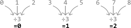
Ushbu o'zgartirilgan indekslar bilan, har bir kichik to'r uchun bitta bo'lgan to'qqizta hash to'plamni 3×3 jadvalda joylashtira olamiz. Bu 3×3 jadvalidagi har bir katakcha bitta kichik to'rga mos keladi.
Bir o'tishda Sudoku tekshiruvi Endi bir o'tishli yechim uchun kerakli barcha narsa mavjud. Hash to'plamlarini qatorlar, ustunlar va kichik to'rlar uchun ishga tushirish bilan boshlaymiz.
To'rdagi har bir katakdan o'tganimizda, joriy qator, ustun va kichik to'rdagi hash to'plamlarda ilgari uchratilgan son mavjudligini tekshiramiz.
- Agar son ushbu hash to'plamlardan birortasida bo'lsa, false qaytaring.
- Aks holda, uni mos qator, ustun va kichik to'r hash to'plamlariga qo'shing.
Bu jarayon har bir qator, ustun va kichik to'rdagi sonlarni kuzatishga yordam beradi. Agar taxtani muvaffaqiyatli ko'rib chiqsak, true qaytaramiz.
Amalga oshirish
from typing import List

def verify_sudoku_board(board: List[List[int]]) -> bool:
    # Create hash sets for each row, column, and subgrid to keep track of numbers
    # previously seen on any given row, column, or subgrid.
    row_sets = [set() for _ in range(9)]
    column_sets = [set() for _ in range(9)]
    subgrid_sets = [[set() for _ in range(3)] for _ in range(3)]
    for r in range(9):
        for c in range(9):
            num = board[r][c]
            if num == 0:
                continue
            # Check if 'num' has been seen in the current row, column, or subgrid.
            if num in row_sets[r]:
                return False
            if num in column_sets[c]:
                return False
            if num in subgrid_sets[r // 3][c // 3]:
                return False
            # If we passed the above checks, mark this value as seen by adding it to
            # its corresponding hash sets.
            row_sets[r].add(num)
            column_sets[c].add(num)
            subgrid_sets[r // 3][c // 3].add(num)
    return True
Murakkablik Tahlili
Bu masalada taxtaning uzunligi 9 ga belgilangan, bu barcha yondashuvlarni vaqt va xotira murakkabligi jihatidan O(1) ga samarali ravishda qisqartiradi.
Vaqt murakkabligi: verify_sudoku_board ning vaqt murakkabligi O(n²), chunki n²=81 ta katakning har birini bir marta ko'rib chiqamiz.
Xotira murakkabligi: row_sets, column_sets va subgrid_sets massivlari sababli xotira murakkabligi O(n²).
Nol Bo'yalishi
Nol Bo'yalishi
m×n matritasadagi har bir nol uchun uning butun qatori va ustunini o'z joyida nolga aylantiring.
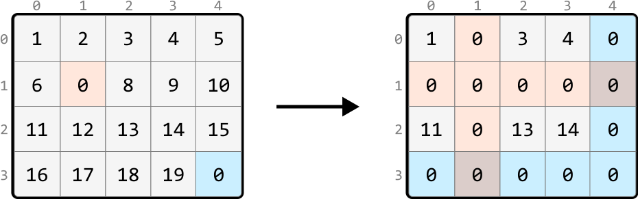
Intuitsiya - Hash To'plamlar
Qo'pol kuch yechimi matritsa dastlab barcha 0 pozitsiyalarini yozib olish va har bir 0 uchun uning qatori va ustunidagi barcha katakchalarni takrorlashni o'z ichiga oladi.
Matritisadagi ixtiyoriy katakchani tasavvur qiling. Matritsa o'zgartirilgandan so'ng, bu katakcha o'z asl qiymatini saqlab qoladi yoki nolga aylanadi.
Asosiy kuzatuv shundan iboratki, agar katakcha nol o'z ichiga oluvchi qator yoki ustunda bo'lsa, u nolga aylanadi.
Katakchaning qatori va ustunida nol borligini tekshirish uchun uni qidirish O(m+n) vaqt oladi. Lekin, barcha qator yoki ustunlarni ikki alohida hash to'plamda saqlash orqali qidirishni O(1) ga qisqartira olamiz.
Bu hash to'plamlar yaratilgandan so'ng, keyingi qadam ularni to'ldirishdir. Matritsa bo'ylab aylanib, nol o'z ichiga oluvchi katakchaga duch kelganimizda:
- Uning qator indeksini qator hash to'plamiga qo'shing (zero_rows).
- Uning ustun indeksini ustun hash to'plamiga qo'shing (zero_cols).
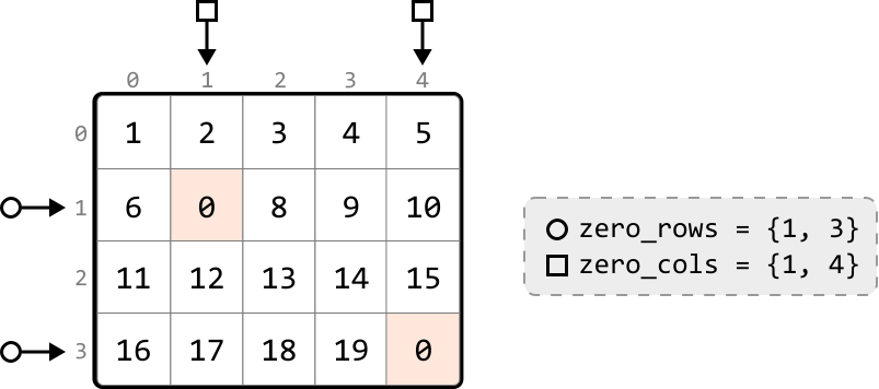
Keyingi, mos hash to'plamlarda qator yoki ustun indekslari mavjud bo'lgan katakchalarni aniqlab ularning qiymatlarini nolga o'zgartiring.
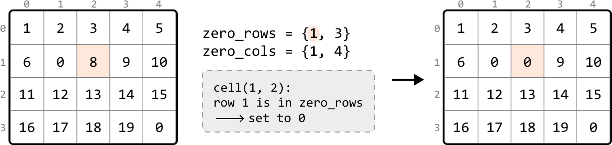
Bu umumiy strategiyani beradi:
- Matritsaning birinchi o'tishida nol o'z ichiga oluvchi har bir katakchani aniqlang va uning qator va ustun indekslarini zero_rows va zero_cols ga qo'shing.
- Ikkinchi o'tishda, qator indeksi zero_rows da yoki ustun indeksi zero_cols da bo'lgan ixtiyoriy katakchani nolga o'rnating.
Amalga oshirish - Hash To'plamlar
from typing import List

def zero_striping_hash_sets(matrix: List[List[int]]) -> None:
    if not matrix or not matrix[0]:
        return
    m, n = len(matrix), len(matrix[0])
    zero_rows, zero_cols = set(), set()
    # Pass 1: Traverse through the matrix to identify the rows and columns
    # containing zeros and store their indexes in the appropriate hash sets.
    for r in range(m):
        for c in range(n):
            if matrix[r][c] == 0:
                zero_rows.add(r)
                zero_cols.add(c)
    # Pass 2: Set any cell in the matrix to zero if its row index is in 'zero_rows'
    # or its column index is in 'zero_cols’.
    for r in range(m):
        for c in range(n):
            if r in zero_rows or c in zero_cols:
                matrix[r][c] = 0
Murakkablik Tahlili
Vaqt murakkabligi: zero_striping_hash_sets ning vaqt murakkabligi O(m·n), chunki biz matritsani ikki marta ko'rib chiqamiz.
Xotira murakkabligi: Nollarni kuzatish uchun ishlatiladigan hash to'plamlarning o'sishi sababli xotira murakkabligi O(m+n): biri qator uchun, ikkinchisi ustun uchun.
Intuitsiya - O'z Joyida Nol Kuzatish
Oldingi yechim asosan hash to'plamlardan foydalanish tufayli vaqt jihatidan samarali edi. Biroq, bu qo'shimcha xotira sarfiga olib keldi.
Muhim kuzatuv shundan iboratki, agar qator yoki ustunda nol bo'lsa, o'sha qator yoki ustandagi barcha katakchalar oxir-oqibat nolga almashtiriladi.
Sinab ko'rishimiz mumkin bo'lgan strategiya — birinchi qator va ustundan (0-qator va 0-ustun) qaysi qator va ustunlar nolga almashinishi kerakligini belgilash uchun belgi sifatida foydalanishdir.
Bu qanday ishlashini tushunish uchun quyidagi misolni ko'rib chiqing. Qatorlar uchun nol o'z ichiga oluvchi qatorlarni belgilash uchun birinchi ustundan foydalanishimiz mumkin:
Qatorlarni qanday belgilaganimizga o'xshab, birinchi qatordan foydalanib nol o'z ichiga oluvchi ustunlarni belgilashimiz mumkin:
Birinchi qator va ustun uchun belgilarni o'rnatish uchun, birinchi qator va ustunni chiqarib, qolgan matritsani qidirish bilan boshlashimiz mumkin.
Endi quyi matritsa katakchalarini ularning mos belgileriga asosan nolga aylantirishni boshlashimiz kerak. Quyi matritsa katakchasi haqida quyidagilarni baholashimiz mumkin:
- Birinchi ustundagi mos belgisi nolmi.
- Birinchi qatordagi mos belgisi nolmi.
Agar bu shartlardan biri bajarilsa, o'sha katakchaning qiymatini nolga o'rnatishimiz kerak:
Ushbu quyi matritsani yangilash uchun ikkinchi qator va ustundan boshlab takrorlashimiz va hozirgina muhokama qilgan mantiqqa asosan katakcha qiymatlarini yangilashimiz mumkin.
Birinchi qator va ustandagi nollarni boshqarish Oldingi bosqichni tugatgandan so'ng, hal qilinishi kerak bo'lgan bitta muammo qoladi. Agar birinchi qator yoki ustunda nol mavjud bo'lsa nima bo'ladi?
Bu yerda birinchi qatordagi qaysi nol dastlabki, qaysi biri belgi sifatida ishlatilgan ekanligini ajratib bo'lmaydi.
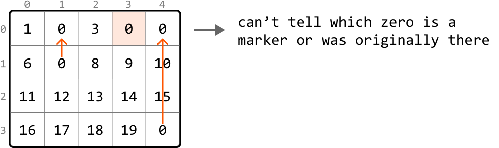
Buning davo usuli — ularni belgi sifatida ishlatishdan oldin birinchi qator yoki ustunda nol mavjudligini belgilaydigan flag o'rnatishdir.
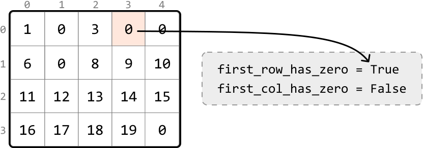
Birinchi qator va ustunni belgilar bilan to'ldirganidan so'ng va mos katakcha qiymatlarini o'rnatgandan keyin, birinchi qator va ustunni keyingi bosqichda yangilashimiz mumkin.
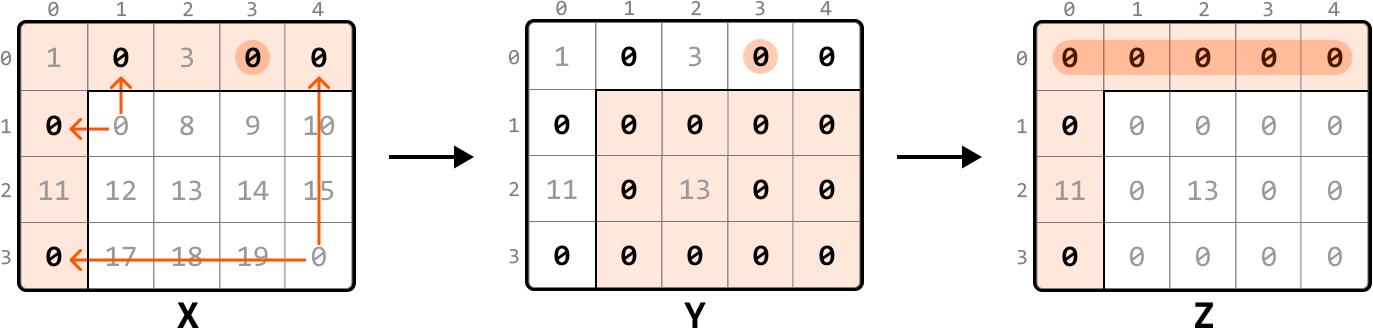
O'z joyida nol belgilash strategiyasi Yuqoridagi yondashuvni quyidagi qadamlarga xulosalaymiz:
- Birinchi qator dastlab nol o'z ichiga oladimi yoki yo'qligini ko'rsatuvchi flag ishlating.
- Birinchi ustun dastlab nol o'z ichiga oladimi yoki yo'qligini ko'rsatuvchi flag ishlating.
- Quyi matritsani ko'rib chiqing, nol o'z ichiga oluvchi qatorlar va ustunlar uchun belgi bo'lib xizmat qilish uchun birinchi qator va ustandagi nollarni o'rnating.
- Belgilarga asosan nollarni qo'llang: ikkinchi qator va ikkinchi ustundan boshlanadigan quyi matritsani ko'rib chiqing. Har bir katakcha uchun uning birinchi qatordagi yoki birinchi ustundagi mos belgisi nol bo'lsa, katakchani nolga o'rnating.
- Agar birinchi qator dastlab nol o'z ichiga olishi belgilangan bo'lsa, birinchi qatordagi barcha elementlarni nolga o'rnating.
- Agar birinchi ustun dastlab nolga ega bo'lishi belgilangan bo'lsa, birinchi ustandagi barcha elementlarni nolga o'rnating.
Amalga oshirish - O'z Joyida Nol Kuzatish
from typing import List

def zero_striping(matrix: List[List[int]]) -> None:
   if not matrix or not matrix[0]:
       return
   m, n = len(matrix), len(matrix[0])
   # Check if the first row initially contains a zero.
   first_row_has_zero = False
   for c in range(n):
       if matrix[0][c] == 0:
           first_row_has_zero = True
           break
   # Check if the first column initially contains a zero.
   first_col_has_zero = False
   for r in range(m):
       if matrix[r][0] == 0:
           first_col_has_zero = True
           break
   # Use the first row and column as markers. If an element in the submatrix is zero,
   # mark its corresponding row and column in the first row and column as 0.
   for r in range(1, m):
       for c in range(1, n):
           if matrix[r][c] == 0:
               matrix[0][c] = 0
               matrix[r][0] = 0
   # Update the submatrix using the markers in the first row and column.
   for r in range(1, m):
       for c in range(1, n):
           if matrix[0][c] == 0 or matrix[r][0] == 0:
               matrix[r][c] = 0
   # If the first row had a zero initially, set all elements in the first row to
   # zero.
   if first_row_has_zero:
       for c in range(n):
           matrix[0][c] = 0
   # If the first column had a zero initially, set all elements in the first column
   # to zero.
   if first_col_has_zero:
       for r in range(m):
           matrix[r][0] = 0
Murakkablik Tahlili
Vaqt murakkabligi: zero_striping ning vaqt murakkabligi O(m·n). Sababi:
- Birinchi qatorni nollar uchun tekshirish O(m) vaqt oladi va birinchi ustunni tekshirish O(n) vaqt oladi.
- Keyin, biz matritsani ikki marta ko'rib chiqamiz: biri 0 larni belgilash uchun, ikkinchisi bu belgilarga asosan matritsani yangilash uchun.
- Nihoyat, birinchi qator va birinchi ustunni bir marta ko'rib chiqamiz, bu O(m) va O(n) vaqt oladi.
Shuning uchun umumiy vaqt murakkabligi O(m)+O(n)+O(m·n)=O(m·n).
Xotira murakkabligi: Biz qaysi qatorlar va ustunlar nolga o'rnatilishi kerakligini kuzatish uchun birinchi qator va ustunni belgi sifatida ishlatsak, xotira murakkabligi O(1).
Ketma-ket Sonlarning Eng Uzun Zanjiri
Ketma-ket Sonlarning Eng Uzun Zanjiri
Massivdagi ketma-ket sonlarning eng uzun zanjirini toping. Farqi 1 bo'lgan ikki son ketma-ket hisoblanadi.
Misol:
Input: nums = [1, 6, 2, 5, 8, 7, 10, 3]
Output: 4
Tushuntirish: Ketma-ket sonlarning eng uzun zanjiri 5, 6, 7, 8.
Intuitsiya
Bu masalaga sodda yondashuv — massivni tartiblashdir. Barcha sonlar o'sish tartibida joylashtirilganda, ketma-ket sonlar qo'shni bo'ladi.
![Image represents a visual depiction of a sorting algorithm's effect on an array of numbers. The diagram begins with an unsorted array `[1 6 2 5 8 7 10 3]` enclosed in square brackets. A right-pointing arrow labeled 'sort' indicates a transformation. The result of the sorting operation is shown as two sub-arrays. The first, a peach-colored sub-array `[1 2 3]`, contains the smallest three numbers from the original array. The second, a light-green sub-array `[5 6 7 8 10]`, contains the remaining numbers, which are larger than those in the first sub-array. The label 'longest' is placed above the second sub-array, indicating that this sub-array represents the longest increasing subsequence within the original unsorted array. The entire output is presented as a sequence of numbers within square brackets.](https://bytebytego.com/images/courses/coding-patterns/hash-maps-and-sets/longest-chain-of-consecutive-numbers/image-02-04-1-WPQHUSEG.svg?dpl=dpl_Gs7zfM6MUzjTBjcjps1LqXtb9QmD)
Bu yondashuv tartiblashni talab qiladi, bu O(n log(n)) vaqt oladi, bu yerda n massiv uzunligini bildiradi.
Shuni tushunish muhimki, massivdagi har bir son ba'zi ketma-ket zanjirning boshini ifodalashi mumkin. Bir yondashuv — har bir sonni potentsial zanjir boshi sifatida ko'rib chiqish va u boshlaydigan zanjirning uzunligini hisoblashdir.
Buni amalga oshirish uchun, ixtiyoriy num son uchun keyingi ketma-ket son num + 1 bo'lishini ta'minlashdan foydalanishimiz mumkin. Bu sonlarni hash to'plamda saqlash orqali tezkor qidirishni amalga oshirish imkonini beradi.
from typing import List

def longest_chain_of_consecutive_numbers_brute_force(nums: List[int]) -> int:
    if not nums:
        return 0
    longest_chain = 0
    # Look for chains of consecutive numbers that start from each number.
    for num in nums:
        current_num = num
        current_chain = 1
        # Continue to find the next consecutive numbers in the chain.
        while (current_num + 1) in nums:
            current_num += 1
            current_chain += 1
        longest_chain = max(longest_chain, current_chain)
    return longest_chain
Bu qo'pol kuch yondashuvi O(n³) vaqt oladi, chunki ichki o'rnatilgan operatsiyalar mavjud:
- Tashqi for-tsikl har bir elementni ko'rib chiqadi, bu O(n) vaqt oladi.
- Har bir element uchun ichki while-tsikl uzoq ketma-ket ketma-ketlik mavjud bo'lsa n tagacha iteratsiya qilishi mumkin.
- Har bir while-tsikl iteratsiyasi uchun massivda keyingi ketma-ket son borligini tekshirish uchun O(n) tekshiruvi bajariladi.
Bu tartiblash yondashuvidan sekinroq, lekin vaqt murakkabligini yaxshilash uchun bir nechta optimizatsiya amalga oshirishimiz mumkin.
Optimizatsiya - hash to'plam Ketma-ketlikdagi keyingi sonni topish uchun massiv bo'ylab chiziqli qidiruv bajaramiz. Biroq, sonlarni hash to'plamda saqlash orqali bu qidiruvni O(1) ga tezlashtirishimiz mumkin.
Bu vaqt murakkabligini O(n³) dan O(n²) ga kamaytiradi.
Optimizatsiya - har bir zanjirning boshini aniqlash Qo'pol kuch yondashuvida har bir sonni zanjir boshi sifatida ko'rib chiqamiz. Bu notekis: ba'zi sonlar zanjirning o'rtasida yoki oxirida bo'lishi mumkin.
![Image represents a diagram illustrating a search for a consecutive chain of numbers. The top of the diagram contains the text 'find the rest of a consecutive chain starting at:'. From this text, eight orange arrows point downwards to a set of single-digit numbers enclosed in square brackets: [1, 6, 2, 5, 8, 7, 10, 3]. The arrows visually represent the exploration of potential consecutive chains starting from an unspecified initial number (implied by the phrase 'starting at:'). The numbers at the bottom are potential candidates or elements within the search space for completing the consecutive chain. The diagram suggests a branching or fan-out search strategy, where multiple possibilities are explored simultaneously to find the rest of the consecutive chain.](https://bytebytego.com/images/courses/coding-patterns/hash-maps-and-sets/longest-chain-of-consecutive-numbers/image-02-04-2-G5TFKSHN.svg?dpl=dpl_Gs7zfM6MUzjTBjcjps1LqXtb9QmD)
Asosiy kuzatuv shundan iboratki, zanjiridagi har bir son uchun bu qidiruvni bajarishimiz shart emas. Buning o'rniga, faqat zanjirdagi eng kichik son, ya'ni zanjir boshi uchun qidiruv bajarishimiz kerak.
![Image represents a diagram illustrating the concept of finding a consecutive chain within a sequence of numbers. The top of the diagram displays the text 'find the rest of a consecutive chain starting at:'. Three orange arrows emanate downwards from this text, pointing to three distinct subsequences of numbers: '[1 6 2]', '[5 8 7]', and '[10 3]'. Below each subsequence, grey arrows indicate potential consecutive chains. Specifically, under '[1 6 2]', a grey arrow points to '1 2 3', suggesting a possible consecutive chain starting with 1. Similarly, under '[5 8 7]', a grey arrow points to '5 6 7 8', indicating a potential consecutive chain starting with 5. Finally, under '[10 3]', a grey arrow points to '10', showing a single-element consecutive chain starting at 10. The diagram visually represents the challenge of identifying consecutive number sequences from a larger, unordered set.](https://bytebytego.com/images/courses/coding-patterns/hash-maps-and-sets/longest-chain-of-consecutive-numbers/image-02-04-3-CQL6HS4J.svg?dpl=dpl_Gs7zfM6MUzjTBjcjps1LqXtb9QmD)
Sonning o'z zanjirida eng kichik son ekanligini oldingi sonni massivda borligini tekshirish orqali aniqlay olamiz. Agar oldingi son (num - 1) massivda bo'lmasa, num zanjir boshidir.
![Image represents a step-by-step illustration of an algorithm, likely searching within an array. The top section shows an array `[1, 6, 2, 5, 8, 7, 10, 3]`. The number 5 is highlighted in a grey circle. Above it, text states 'not the smallest in its chain: 6 - 1 = 5 exists,' indicating a check for whether 5 is the smallest element in a sub-array derived by subtracting 1 from a larger element (in this case, 6). A downward-pointing arrow connects this text to the array, visually indicating the element being processed. The bottom section shows the same array, but now the number 5 is no longer highlighted. Above it, the text reads 'smallest in its chain: 5 - 1 = 4 doesn't exist,' implying that a search for 4 (5-1) within the array failed. A downward-pointing arrow again connects the text to the array, showing that the algorithm continues its search after finding that 5 is not the smallest in its chain. The overall image demonstrates a process of iterating through an array and checking for the existence of specific values derived from calculations on other array elements.](https://bytebytego.com/images/courses/coding-patterns/hash-maps-and-sets/longest-chain-of-consecutive-numbers/image-02-04-4-O5NZ7DPG.svg?dpl=dpl_Gs7zfM6MUzjTBjcjps1LqXtb9QmD)
Bu vaqt murakkabligini O(n²) dan O(n) ga kamaytiradi, chunki endi har bir zanjir faqat bir marta qidiruvga tushadi.
Amalga oshirish
from typing import List

def longest_chain_of_consecutive_numbers(nums: List[int]) -> int:
    if not nums:
        return 0
    num_set = set(nums)
    longest_chain = 0
    for num in num_set:
        # If the current number is the smallest number in its chain, search for
        # the length of its chain.
        if num - 1 not in num_set:
            current_num = num
            current_chain = 1
            # Continue to find the next consecutive numbers in the chain.
            while current_num + 1 in num_set:
                current_num += 1
                current_chain += 1
            longest_chain = max(longest_chain, current_chain)
    return longest_chain
Murakkablik Tahlili
Vaqt murakkabligi: longest_chain_of_consecutive_numbers ning vaqt murakkabligi O(n), chunki ichki while-tsikl ham bor bo'lsa-da, har bir element ko'pi bilan ikki marta qayta ishlanadi.
Xotira murakkabligi: Hash to'plam massivdagi har bir noyob sonni saqlashi sababli xotira murakkabligi O(n).
Geometrik Ketma-ketlik Uchliklari
Geometrik Ketma-ketlik Uchliklari
Geometrik ketma-ketlik uchligi — har bir keyingi son oldingi sonni umumiy koeffitsientga ko'paytirish orqali olinadigan uchta sondan iborat ketma-ketlik.
Uchta uchlikni ko'rib chiqaylik:
- (1, 2, 4): Bu koeffitsienti 2 bo'lgan geometrik ketma-ketlik (ya'ni [1, 1·2 = 2, 2·2 = 4]).
- (5, 15, 45): Bu koeffitsienti 3 bo'lgan geometrik ketma-ketlik (ya'ni [5, 5·3 = 15, 15·3 = 45]).
- (2, 3, 4): Geometrik ketma-ketlik emas.
Butun sonlar massivi va umumiy koeffitsient r berilgan, massivda geometrik ketma-ketlikni ifodalovchi barcha (i, j, k) indekslar uchliklarini toping.
Misol:
![Image represents five rows demonstrating a geometric sequence. Each row begins with a bracketed sequence of numbers: [2, 1, 2, 4, 8], with some rows having additional numbers (8) at the end. The numbers 2, 4, and 8 within the brackets are highlighted in peach-colored circles, and small numbers beneath them indicate their position within the sequence (0, 2, 3, 4, 5). Following each bracketed sequence is a colon and then an equation demonstrating the pattern: (2, 2*2 = 4, 4*2 = 8). The first number in the equation (2) corresponds to the first highlighted number in the bracket, and subsequent numbers are generated by multiplying the preceding number by 2. The last row shows a variation where the sequence starts with 1 instead of 2, resulting in a modified equation: (1, 1*2 = 2, 2*2 = 4). The overall image illustrates the concept of a geometric progression where each term is obtained by multiplying the previous term by a constant value (in this case, 2).](https://bytebytego.com/images/courses/coding-patterns/hash-maps-and-sets/geometric-sequence-triplets/geometric-sequences-triplets-ZJZMJ6MD.svg?dpl=dpl_Gs7zfM6MUzjTBjcjps1LqXtb9QmD)
Input: nums = [2, 1, 2, 4, 8, 8], `r` = 2
Output: 5
Tushuntirish:
- [2, 4, 8] uchligi (0, 3, 4), (0, 3, 5), (2, 3, 4), (2, 3, 5) indekslarida uchraydi.
- [1, 2, 4] uchligi (1, 2, 3) indekslarida uchraydi.
Intuitsiya
Uchlik geometrik ketma-ketlikni hosil qilishi uchun ikki asosiy qoidaga amal qilishi kerak:
- U umumiy koeffitsient r bilan geometrik ketma-ketlikka amal qiladigan uchta qiymatdan iborat.
- Uchlikni hosil qiluvchi uchta qiymat massivda geometrik ketma-ketlikdagi kabi tartibda bo'lishi kerak.
Geometrik ketma-ketlikni 1-qoidaga mos kelishi uchun qanday ifodalashimiz mumkin? Birinchi son x deylik. Ikkinchi son x·r, uchinchi son esa x·r² bo'ladi.
Qo'pol kuch yondashuvi — massivdagi har bir mumkin bo'lgan uchlikni ko'rib chiqib ulardan qaysi biri geometrik ketma-ketlikka mos kelishini tekshirishdir.
Bu yerda muhim kuzatuv shundan iboratki, agar uchlikning bir qiymatini bilsak, boshqa ikki qiymat nima bo'lishi kerakligini hisoblay olamiz.
Chunki barcha uchta qiymat umumiy koeffitsient r bilan bog'langan. Shuning uchun massivdagi ixtiyoriy x son uchun faqat x/r va x·r qiymatlarini topishimiz kerak.
![Image represents a diagram illustrating an ordering problem in a data structure. A single 'X' at the top points downwards via a grey arrow to a horizontal array-like structure enclosed in square brackets `[ ]`. This array contains several elements represented by dots (`.`) as placeholders, with a single 'X' and then 'x*r²' and 'x*r' appearing in the array. Below the array, a grey box highlights the text '(x, x*r², x*r)' labeled as 'triplet valves,' indicating that these three elements are expected to form a triplet. The text 'appear in the wrong order' explains that the order of these elements within the array does not match the expected order defined in the triplet valves. The diagram visually shows the incorrect arrangement of the triplet within a larger data structure, highlighting the problem of out-of-order elements.](https://bytebytego.com/images/courses/coding-patterns/hash-maps-and-sets/geometric-sequence-triplets/image-02-05-1-752GC5NK.svg?dpl=dpl_Gs7zfM6MUzjTBjcjps1LqXtb9QmD)
Bu muammoni (x/r, x, x·r) uchlik ko'rinishi yordamida hal qilishimiz mumkin, bu doimo tartibni saqlash imkonini beradi.

x/r va x·r qiymatlarini topishning bir usuli — chap va o'ng quyi massivlar bo'ylab chiziqli qidiruvdir. Bu chiziqli qidiruv uchlik boshiga O(n) sarflaydi.
Hash xaritalar Hash xarita bu masalani hal qilish uchun zo'r, chunki u doimiy vaqtda ma'lum qiymatlarni qidirish imkonini beradi.
Kerak bo'ladigan ikkita hash xarita:
- Har bir x ning chap tomonidagi sonlarni o'z ichiga oluvchi hash xarita (left_map).
- Har bir x ning o'ng tomonidagi sonlarni o'z ichiga oluvchi hash xarita (right_map).
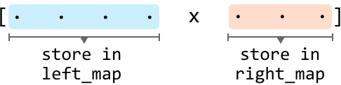
Hash xaritalar chap hash xaritadan x/r ni va o'ng hash xaritadan x·r ni doimiy vaqtda so'rash imkonini beradi.
Barcha (x/r, x, x·r) uchliklarini topish Maqsadimiz geometrik ketma-ketlikka amal qiladigan barcha uchliklarni topish, har birini (x/r, x, x·r) sifatida ifodalamoqda.
Uchlikning x/r qiymatini topishdan oldin x ning r ga bo'linishini tekshirishimiz kerak. Agar bo'linmasa, triplet hosil qilib bo'lmaydi.
Ixtiyoriy x element uchun left_map da bir nechta x/r nusxasi va right_map da bir nechta x·r nusxasi bo'lishi mumkin.
![Image represents a diagram illustrating a coding pattern, possibly related to data structures or algorithms. The diagram shows two parallel structures, each representing a set of numbers. The left structure, labeled 'x/r = 2' in light blue, depicts a set [2, 1, 2], where two instances of the number 2 are connected by a line labeled 'two 2's' to a central node. The right structure, labeled 'x/r = 8' in orange, shows a set [8, 8], with two instances of 8 connected by a line labeled 'two 8's' to the same central node. A downward-pointing arrow labeled 'x' connects the two structures, indicating a transformation or operation. The central node, connected to both structures, is labeled '2 * 2 = 4', suggesting a calculation based on the number of instances in each structure. Finally, an arrow pointing to the right indicates the result: '4 instances of [2, 4, 8]', implying that the combined result of the operation on the two input structures produces four instances of the combined set [2, 4, 8].](https://bytebytego.com/images/courses/coding-patterns/hash-maps-and-sets/geometric-sequence-triplets/image-02-05-4-ZCKYY7SP.svg?dpl=dpl_Gs7zfM6MUzjTBjcjps1LqXtb9QmD)
Bu umumiy metodologiyani quyidagi qadamlarga xulosalash mumkin:
![Image represents a flowchart illustrating a coding pattern for counting triplets. The top shows two arrays, a light-blue array labeled `[`...`]` on the left representing values of `x/r`, and a peach-colored array labeled `[`...`]` on the right representing values of `x*r`, separated by the variable 'x'. Step ①, labeled 'check that x%r == 0', indicates a condition that must be met. Step ②, labeled 'get frequency of x/r from left_map', shows an arrow pointing from the left array to step ④. Similarly, step ③, labeled 'get frequency of x*r from right_map', shows an arrow pointing from the right array to step ④. Step ④, labeled 'multiply the frequencies to get the number of triplets with this x in the middle', indicates that the frequencies obtained in steps ② and ③ are multiplied to determine the count of triplets where 'x' is the central element, satisfying the condition in step ①. The arrows visually represent the data flow, showing how the frequencies from the left and right arrays are combined to calculate the final result.](https://bytebytego.com/images/courses/coding-patterns/hash-maps-and-sets/geometric-sequence-triplets/image-02-05-5-BXUCZYYO.svg?dpl=dpl_Gs7zfM6MUzjTBjcjps1LqXtb9QmD)
E'tibor bering, agar x/r yoki x·r ularning hash xaritalarida topilmasa, ularning chastotasi standart ravishda 0.
Keling, quyidagi misol yordamida bu strategiyani amalga oshiraylik:
![Image represents a one-dimensional array or list enclosed in square brackets `[` and `]`, containing the integer sequence `[2, 1, 2, 4, 8, 8]`. This array is separated by a comma from the assignment `r = 2`, indicating a variable `r` is assigned the integer value 2. The arrangement shows the array as a data structure, and the assignment suggests a potential relationship between the array and the variable `r`, possibly representing a parameter or index related to the array's processing or manipulation within a larger algorithm or code. There are no URLs or other parameters present beyond the numerical values and variable assignment.](https://bytebytego.com/images/courses/coding-patterns/hash-maps-and-sets/geometric-sequence-triplets/image-02-05-6-UWRMOSID.svg?dpl=dpl_Gs7zfM6MUzjTBjcjps1LqXtb9QmD)
Hash xaritalar har doim to'g'ri qiymatlarni o'z ichiga olishini ta'minlash uchun yangilashni o'z ichiga oluvchi dinamik strategiyani kiritishimiz kerak.
Massivni chapdan o'ngga ko'rib chiqayotganligi sababli, right_map ni dastlab massivdagi barcha qiymatlar bilan to'ldirishimiz kerak.
![Image represents a visual depiction of a data transformation process, likely related to frequency counting or mapping. The input is a list of numbers `[2, 1, 2, 4, 8, 8]` and a value `r = 2`. This input is processed to generate two maps: `left_map` and `right_map`. `right_map` is a table with two columns: `x*r` and `freq`. It shows the results of multiplying each element in the input list by `r` (2) in the `x*r` column, and the frequency of each resulting value in the `freq` column. For example, 2*2=4 appears once, 1*2=2 appears twice, 4*2=8 appears twice. `left_map` is an empty table with columns `x/r` and `freq`, suggesting it would contain the results of dividing each input element by `r` and their corresponding frequencies, but these values are not shown in the image. The overall diagram illustrates a process where an input list is transformed based on a given value `r`, resulting in frequency counts displayed in two separate tables representing different operations (multiplication and division by `r`).](https://bytebytego.com/images/courses/coding-patterns/hash-maps-and-sets/geometric-sequence-triplets/image-02-05-7-TYGFBIEY.svg?dpl=dpl_Gs7zfM6MUzjTBjcjps1LqXtb9QmD)
Endi uchliklarni qidiraylik. Birinchi qiymatni uchlikning o'rta qiymati (x) sifatida ifodalashdan boshlaylik.
Avval right_map ni yangilaymiz. Joriy qiymat (2) ni right_map dan olib tashlaymiz, chunki bu 2 ni o'ng tomonida emas.
![Image represents a diagram illustrating a coding pattern, possibly related to frequency counting or mapping. The diagram shows an input array `x = [2, 1, 2, 4, 8, 8]` and a value `r = 2`. This input is processed to create two maps: `left_map` and `right_map`. `left_map` is empty, suggesting it's a placeholder or the result of a computation not yet shown. `right_map` is a table with two columns: `x*r` (representing elements of the input array multiplied by `r`) and `freq` (representing the frequency of each element in `x*r`). The `right_map` contains the following entries: `x*r` values of 2, 1, 4, 8 and their corresponding frequencies in `freq` as 2, 1, 1, 2 respectively. An arrow points from the `freq` column value of 2 (corresponding to `x*r` = 2) to the number 1, indicating a potential further processing step or mapping not fully depicted. The overall structure suggests a process where an input array is manipulated based on a given value `r`, resulting in frequency counts displayed in the `right_map`, with a possible additional transformation indicated by the arrow.](https://bytebytego.com/images/courses/coding-patterns/hash-maps-and-sets/geometric-sequence-triplets/image-02-05-8-5GDFYZ4K.svg?dpl=dpl_Gs7zfM6MUzjTBjcjps1LqXtb9QmD)
Keyingi, x/r butun son ekanligini tekshiramiz. Bu holda shunday, shuning uchun x ni o'rta son sifatida olgan uchliklar sonini topaylik.
![The image represents a code snippet illustrating a calculation process. On the left, an array `[2 1 2 4 8 8]` is shown, with a variable `r` assigned the value 2. A downward-pointing arrow suggests this array is input to the process. On the right, a light-grey box contains a conditional statement and a series of calculations. The condition `x % r == 0` checks if a variable `x` (not explicitly defined in the image but implied to be an element from the input array) is divisible by `r`. If true, the `count` variable is updated. The update involves multiplying values from two maps, `left_map` and `right_map`, using `x/r` and `x*r` as indices respectively. The example shows the calculation for `x=2`, resulting in `count += left_map[2/2] * right_map[2*2]`, which simplifies to `count += left_map[1] * right_map[4]`. Subsequent lines show further additions to `count`, ultimately resulting in `count += 0`, suggesting that the initial multiplication resulted in zero, and subsequent additions also contributed zero. The overall structure depicts a conditional update of a counter based on array elements and lookups in two maps (`left_map` and `right_map`).](https://bytebytego.com/images/courses/coding-patterns/hash-maps-and-sets/geometric-sequence-triplets/image-02-05-9-OAMR6D5N.svg?dpl=dpl_Gs7zfM6MUzjTBjcjps1LqXtb9QmD)
Keyingi qiymatga o'tishdan oldin joriy sonni left_map ga qo'shamiz, chunki u endi potentsial x/r bo'lib qoladi.
Bu jarayonni massivning qolgan qismi uchun takrorlash r koeffitsientli barcha geometrik uchliklarni topish imkonini beradi.
![Image represents a diagram illustrating a coding pattern, possibly related to data processing or algorithm design. At the top, an input array `[2 1 2 4 8 8]` and a parameter `r = 2` are shown. A downward-pointing arrow indicates the processing of the input array. Below, two tables are presented side-by-side, labeled 'left_map' and 'right_map'. 'left_map' contains a column labeled 'x/r' with values (presumably resulting from dividing elements of the input array by `r`) and a column labeled 'freq' representing their frequencies. Similarly, 'right_map' has columns 'x*r' (likely representing multiplication of input array elements by `r`) and 'freq' showing their frequencies. A light gray rectangular box displays the condition `x % r != 0 → can't form a triplet → continue`, indicating that if the remainder of an element divided by `r` is not zero, a triplet cannot be formed, and the process continues to the next element. The overall diagram suggests a frequency analysis or counting process involving division and multiplication by a given parameter `r`, with a conditional check for triplet formation.](https://bytebytego.com/images/courses/coding-patterns/hash-maps-and-sets/geometric-sequence-triplets/image-02-05-11-7SP3U7QX.svg?dpl=dpl_Gs7zfM6MUzjTBjcjps1LqXtb9QmD)
![Image represents a diagram illustrating a coding pattern, possibly related to frequency counting or data manipulation. At the top, an input array `[2 1 2 4 8 8]` and a value `r = 2` are given. Below, two tables labeled 'left_map' and 'right_map' are shown. 'left_map' contains two columns: 'x/r' representing values after integer division by `r`, and 'freq' representing their frequencies. Similarly, 'right_map' has columns 'x*r' (values after multiplication by `r`) and 'freq'. The values in these tables seem pre-calculated based on the input array. A dashed-line box to the right shows a calculation process. It starts with a condition `x % r == 0`, implying a check for divisibility by `r`. If true, a `count` variable is updated by adding the product of a value from 'left_map' (indexed by `x/r`) and a value from 'right_map' (indexed by `x*r`). An example calculation is shown, where `x` is implicitly 2, resulting in `left_map[2/2] * right_map[2*2]`, which simplifies to `1 * 1`, adding 1 to the `count`. The entire process suggests an algorithm that uses pre-computed frequency maps ('left_map' and 'right_map') to efficiently process the input array based on divisibility by `r`.](https://bytebytego.com/images/courses/coding-patterns/hash-maps-and-sets/geometric-sequence-triplets/image-02-05-12-F3WBBFPZ.svg?dpl=dpl_Gs7zfM6MUzjTBjcjps1LqXtb9QmD)
![Image represents a diagram illustrating a coding pattern, possibly related to frequency counting or data manipulation. At the top, an input array `[2 1 2 4 8 8]` and a value `r = 2` are given. Below, two tables labeled 'left_map' and 'right_map' are shown. 'left_map' has two columns: 'x/r' (representing the element of the input array divided by r) and 'freq' (frequency). It contains the values 2 (x/r) and 2 (freq) in the first row, and 1 (x/r) and 1 (freq) in the second row. 'right_map' similarly has columns 'x*r' (element multiplied by r) and 'freq', with values 2 and 0, 1 and 0, 4 and 0, and 8 and 2. To the right, a dashed box shows a calculation: `x % r == 0 → count += left_map[x/r] * right_map[x*r]`. This formula is then broken down step-by-step, substituting values from the input array and the maps: `+= left_map[4/2] * right_map[4*2]`, `+= 2 * 2`, and finally `+= 4`, demonstrating how the count is updated based on the values in the 'left_map' and 'right_map' tables. The overall diagram visualizes a process where an input array is processed using two pre-computed frequency maps ('left_map' and 'right_map') to calculate a final count.](https://bytebytego.com/images/courses/coding-patterns/hash-maps-and-sets/geometric-sequence-triplets/image-02-05-13-XPXQHUAJ.svg?dpl=dpl_Gs7zfM6MUzjTBjcjps1LqXtb9QmD)
![Image represents a coding pattern illustration focusing on a calculation involving two maps, `left_map` and `right_map`, and an input array `[2, 1, 2, 4, 8, 8]` with `r` set to 2. An arrow points downwards from 'x' suggesting an input value. `left_map` and `right_map` are presented as tables with two columns: the first labeled 'x/r' or 'x*r' respectively, representing the result of integer division by `r` or multiplication by `r`, and the second labeled 'freq', likely representing frequency counts. The `left_map` contains entries (2,2), (1,1), (4,1), (8,1), while `right_map` contains (2,0), (1,0), (4,0), (8,1). A dashed box to the right shows a calculation process: `x % r == 0` (checking if `x` is a multiple of `r`) leads to `count += left_map[x/r] * right_map[x*r]`. The calculation is further broken down with example values, showing `count` being updated by adding the product of `left_map[8/2]` (which is 1) and `right_map[8*2]` (which is 1), resulting in a final `count` of 0. The diagram illustrates how the maps are used to perform a calculation based on the input array and the value of `r`.](https://bytebytego.com/images/courses/coding-patterns/hash-maps-and-sets/geometric-sequence-triplets/image-02-05-14-TG7MSPTM.svg?dpl=dpl_Gs7zfM6MUzjTBjcjps1LqXtb9QmD)
![Image represents a diagram illustrating a coding pattern, possibly for counting occurrences based on modulo operation. At the top, an input array `[2 1 2 4 8 8]` and a value `r = 2` are given. Below, two tables labeled 'left_map' and 'right_map' are shown side-by-side. Each table has two columns: the first column in 'left_map' lists the elements of the input array divided by `r` (integer division), while the second column represents their frequencies. Similarly, 'right_map' has its first column listing elements of the input array multiplied by `r`, and the second column showing their frequencies. A dashed-line box to the right contains a calculation sequence. It starts with a condition `x % r == 0`, indicating that if an element `x` modulo `r` equals 0, a counter (`count`) is updated. The update involves multiplying the frequency from 'left_map' (using the integer division of `x` by `r` as the index) with the frequency from 'right_map' (using `x` multiplied by `r` as the index). The example calculation shows how this is done for the element 8: `left_map[8/2]` (which is 1) is multiplied by `right_map[8*2]` (which is 0), resulting in 0 being added to the counter. The final result of the calculation is 0 in this specific example.](https://bytebytego.com/images/courses/coding-patterns/hash-maps-and-sets/geometric-sequence-triplets/image-02-05-15-ICJE5233.svg?dpl=dpl_Gs7zfM6MUzjTBjcjps1LqXtb9QmD)
Amalga oshirish
from typing import List
from collections import defaultdict

def geometric_sequence_triplets(nums: List[int], r: int) -> int:
    # Use 'defaultdict' to ensure the default value of 0 is returned when
    # accessing a key that doesn’t exist in the hash map. This effectively sets
    # the default frequency of all elements to 0.
    left_map = defaultdict(int)
    right_map = defaultdict(int)
    count = 0
    # Populate 'right_map' with the frequency of each element in the array.
    for x in nums:
        right_map[x] += 1
    # Search for geometric triplets that have x as the center.
    for x in nums:
        # Decrement the frequency of x in 'right_map' since x is now being
        # processed and is no longer to the right.
        right_map[x] -= 1
        if x % r == 0:
            count += left_map[x // r] * right_map[x * r]
        # Increment the frequency of x in 'left_map' since it'll be a part of the
        # left side of the array once we iterate to the next value of `x`.
        left_map[x] += 1
    return count
Murakkablik Tahlili
Vaqt murakkabligi: geometric_sequence_triplets ning vaqt murakkabligi O(n), chunki nums massivini bir marta ko'rib chiqamiz.
Xotira murakkabligi: Hash xaritalar n gacha o'sishi mumkinligi sababli xotira murakkabligi O(n).
Bog'liq Ro'yxatlar
Bog'liq Ro'yxatlarga Kirish
Bog'liq Ro'yxatlarga Kirish
Intuitsiya
Bog'liq ro'yxat — har bir tugun ketma-ketlikdagi keyingi tugunga bog'langan tugunlar ketma-ketligidan iborat ma'lumotlar strukturasi.
Quyida ko'rsatilganidek ListNode sinfidan foydalanib tugunni aniqlaymiz:
class ListNode:
   def __init__(self, val: int, next: ListNode):
       self.val = val
       self.next = next
Bir yo'nalishli bog'liq ro'yxat
Bog'liq ro'yxatning eng oddiy shakli — bir yo'nalishli bog'liq ro'yxat, bunda har bir tugun keyingi tugunga ishora qiladi.

Bog'liq ro'yxatdagi boshqa tugunlarga kirish uchun bosh (head) dan boshlab uni kesib o'tishimiz kerak.

Bir yo'nalishli bog'liq ro'yxatlar ma'lumotlar to'plamini saqlash uchun ishlatilishi mumkin. Ularning asosiy afzalligi — bosh va oxiridagi kiritish va o'chirish amallari O(1) da bajarilishi.
Ushbu amallarning samaradorligi tasodifiy kirishni amalga oshirishning imkonsizligi hisobiga keladi, chunki tugunlar xotirada ketma-ket joylashmagan.
Ikki yo'nalishli bog'liq ro'yxat Ikki yo'nalishli bog'liq ro'yxat — har bir tugun ham keyingi, ham oldingi tugunga ko'rsatkichga ega bo'lgan bog'liq ro'yxatning kengaytirilgan versiyasi.

Ikki yo'nalishli bog'liq ro'yxatning katta afzalligi — ikki tomonlama kesib o'tish imkoniyatidir. Bundan tashqari, ikki yo'nalishli bog'liq ro'yxatlar o'rtadagi tugunni O(1) da o'chirish imkonini beradi.
Ko'rsatkich Manipulyatsiyasi
Ko'plab bog'liq ro'yxat intervyu masalalari bog'liq ro'yxatni kesib o'tish yoki qayta tuzishni talab qiladi. Ko'rsatkich manipulyatsiyasini tushunish bu masalalar uchun juda muhim.
Hayotiy Misol
Musiqa o'ynatish ro'yxati: Musiqa pleyer ilovalari ko'pincha o'ynatish ro'yxatlarini amalga oshirish uchun bog'liq ro'yxatlardan foydalanadi.
Bob Mazmuni
Bu bobda bir yo'nalishli va ikki yo'nalishli bog'liq ro'yxatlarni o'z ichiga olgan masalalarni ko'rib chiqamiz.
Bog'liq Ro'yxatni Teskari Aylantirish
Bog'liq Ro'yxatni Teskari Aylantirish
Bir yo'nalishli bog'liq ro'yxatni teskari aylantiring.
Misol:
Intuitsiya - Iterativ
Sodda strategiya — bog'liq ro'yxat qiymatlarini massivda saqlash va bog'liq ro'yxatni qayta tiklashdir. Lekin bu O(n) qo'shimcha xotira talab qiladi.
Masalani ko'rsatkich manipulyatsiyasi nuqtai nazaridan ko'rib chiqaylik. Asosiy kuzatuv shundan iboratki, agar ko'rsatkichlarning yo'nalishini o'zgartirsak, bog'liq ro'yxat teskari bo'ladi.
Endi ushbu ko'rsatkich manipulyatsiyasini qanday amalga oshirishni aniqlashimiz kerak. Quyidagi misolni ko'rib chiqing.

Barcha ko'rsatkichlarning yo'nalishini teskari aylantirish uchun tugunlarni birma-bir takrorlaymiz. Bu jarayonda curr_node ni joriy tugunga va prev_node ni oldingi tugunga ishora qiladigan ikkita ko'rsatkich saqlaymiz.

Keyingi ko'rsatkichni teskari aylantirish uchun curr_node va prev_node ko'rsatkichlarini bir tugunga siljitish usulimiz bo'lishi kerak.
Bu curr_node ni teskari aylantirmasdan oldin 2-tugunga havola saqlaganligimiz kerakligini ko'rsatadi. Buni next_node o'zgaruvchisi orqali amalga oshirishimiz mumkin.

E'tibor bering, next_node ni siljitishimiz shart emas, chunki u keyingi iteratsiyada curr_node.next bilan o'rnatilishi mumkin.
Bu mantiqni uch qadamda xulosalashimiz mumkin. Bog'liq ro'yxatdagi har bir tugunga:
- Keyingi tugunga havola saqlang (next_node = curr_node.next).
- Joriy tugunning keyingi ko'rsatkichini oldingi tugunga bog'lang (curr_node.next = prev_node).
- prev_node va curr_node ni bir tugunga oldinga siljiting (prev_node = curr_node, curr_node = next_node).
Keling, bog'liq ro'yxatning qolgan qismi uchun bu qadamlarni takrorlaymiz:






curr_node null ga aylanganda teskari aylantirishni to'xtatishimiz mumkin, bu orqaga qaytariladigan ko'proq tugunlar yo'qligini bildiradi.
So'nggi qadam — teskari aylantirilgan bog'liq ro'yxatning boshini qaytarishdir, bu prev_node ga ishora qiladi.
Amalga oshirish - Iterativ
from ds import ListNode

def linked_list_reversal(head: ListNode) -> ListNode:
    curr_node, prev_node = head, None
    # Reverse the direction of each node's pointer until 'curr_node' is null.
    while curr_node:
        next_node = curr_node.next
        curr_node.next = prev_node
        prev_node = curr_node
curr_node = next_node # 'prev_node' will be pointing at the head of the reversed linked list.
return prev_node
Murakkablik Tahlili
Vaqt murakkabligi: linked_list_reversal ning vaqt murakkabligi O(n), bu yerda n bog'liq ro'yxatdagi tugunlar sonini bildiradi.
Xotira murakkabligi: Xotira murakkabligi O(1).
Intuitsiya - Rekursiv
Ba'zan intervyu olib boruvchi masalani rekursiya yordamida hal qilishni xohlashi mumkin. Rekursiv yechim qanday ko'rinishini ko'rib chiqaylik.
Rekursiv yechimda masala bir xil masalaning kichikroq nusxalarini hal qilish orqali yechiladi. Bog'liq ro'yxatning rekursiv teskari aylantirilishi uchun uni kichikroq bog'liq ro'yxatlarni teskari aylantirish masalasiga qisqartirishimiz kerak.
Ushbu masalaning eng kichik versiyasi 0 yoki 1 o'lchamli bog'liq ro'yxatni teskari aylantirishdir. Bu bog'liq ro'yxatlar allaqachon teskari aylantirilib bo'lingan.
Shu ma'lumotdan foydalanib, quyidagi misol yordamida rekursiv funksiya mantiqini yaratishga harakat qilaylik:
Qaysi quyi masalani hal qilishimiz kerakligini o'ylab ko'ring. Butun bog'liq ro'yxatni teskari aylantirish uchun head.next dan boshlanadigan kichik ro'yxatda linked_list_reversal funksiyamizdan foydalanishimiz mumkin.
Aytilganidek, avval head.next dan boshlanadigan ro'yxatda linked_list_reversal ni rekursiv chaqiraylik.
Rekursiv funksiyani loyihalashda, o'sha funksiyaga ixtiyoriy rekursiv chaqiruv mo'ljallangan tarzda ishlaydi deb faraz qiling.
Keyingi, teskari aylantirilgan quyi ro'yxatning dumini (2-tugun) 1-tugunga ishora qilishi kerak. 2-tugunga head.next orqali murojaat qilishimiz mumkin.

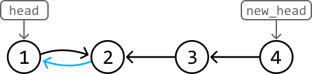
Bog'liq ro'yxat deyarli to'liq teskari aylantirildi, lekin 1-tugun hali 2-tugunga ishora qilmoqda. Buni olib tashlash uchun 1-tugunning keyingi ko'rsatkichini null ga o'rnatamiz.


Amalga oshirish - Rekursiv
from ds import ListNode

def linked_list_reversal_recursive(head: ListNode) -> ListNode:
    # Base cases.
    if (not head) or (not head.next):
        return head
    # Recursively reverse the sublist starting at the next node.
    new_head = linked_list_reversal_recursive(head.next)
    # Connect the reversed sublist to the head node to fully reverse the entire linked list.
    head.next.next = head
    head.next = None
    return new_head
Murakkablik Tahlili
Vaqt murakkabligi: linked_list_reversal_recursive ning vaqt murakkabligi O(n), chunki u n ta rekursiv chaqiruvni o'z ichiga oladi.
Xotira murakkabligi: Rekursiv chaqiruvlar stacki sababli xotira murakkabligi O(n).
Intervyu Maslahat
Maslahat: Ko'rsatkich manipulyatsiyalarini vizuallang. Ko'pincha ko'rsatkichlarni qayerda o'zgartirish kerakligini aniqlash murakkab bo'lishi mumkin.
Bog'liq Ro'yxatdan K-chi Oxirgi Tugunni Olib Tashlash
Bog'liq Ro'yxatdan K-chi Oxirgi Tugunni Olib Tashlash
Bir yo'nalishli bog'liq ro'yxatning oxiridan k-chi tugunni olib tashlaganidan so'ng boshini qaytaring.
Misol:
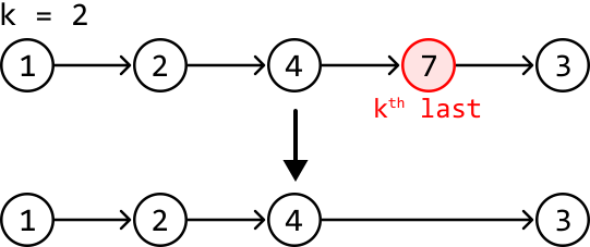
Cheklovlar:
- Bog'liq ro'yxat kamida bitta tugunni o'z ichiga oladi.
Intuitsiya
Bu masalani ikki maqsadga bo'lishimiz mumkin:
- K-chi oxirgi tugunning pozitsiyasini toping.
- Ushbu tugunni olib tashlang.
Avval tugunni olib tashlash qanday ishlashini tushunib olaylik. Quyidagi misolni ko'rib chiqing.

Bu k-chi oxirgi tugunni olib tashlash uchun u oldinidagi tugunni topishimiz kerakligini bildiradi.
Bu masalaga sodda yechim — birinchi marta bog'liq ro'yxatning uzunligini (n) topish va k-chi oxirgi tugunni (n-k)chi tugun sifatida aniqlashdir.
Bir for-tsiklda bir yo'nalishli bog'liq ro'yxatni kesib o'tishning qiyinligi — kesib o'tganda tugunning bog'liq ro'yxatda necha joyga ketishini bilmaslikdir.
Bitta o'rniga ikkita ko'rsatkichdan foydalanishni ko'rib chiqing. Bir ko'rsatkich bog'liq ro'yxat oxiriga yetganida ikkinchisi k-chi oxirgi tugunning oldinidagi tugunga turishi mumkin bo'lgan ssenariy yaratasizmi?

Birinchi ko'rsatkichni leader, uni kuzatib boradiganini esa trailer deb ataymiz. Leader ko'rsatkich oxirga yetganda, trailer ko'rsatkich k-chi oxirgi tugunning oldinidagi tugunga turishi uchun leader ning trailer dan k qadam oldinda bo'lishini xohlaymiz.
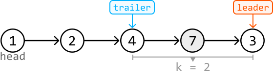
Bunga erishish uchun, avval leader ko'rsatkichni k qadam oldinga siljitamiz. Bu leader ning trailer dan k qadam oldinda bo'lishini ta'minlaydi.
Biroq, avval ko'rib chiqilishi kerak bo'lgan muhim chekka holat mavjud: agar bosh tugunning o'zi olib tashlanishi kerak bo'lsa nima bo'ladi?

Endi strategiyamizni misol bilan qo'llashga harakat qilaylik.
Avval, leader ko'rsatkichni k (2) marta oldinga siljiting, u trailer ko'rsatkichdan k tugun oldinda bo'lsin:
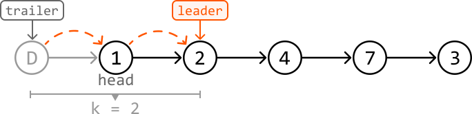
Leader k tugun oldinda bo'lishi bilan, leader oxiriga yetguncha trailer va leader ko'rsatkichlarini bir vaqtda siljitishimiz mumkin.



Trailer ko'rsatkichi ideal pozitsiyada bo'lganida, 7-tugunni olib tashlashimiz mumkin:


Ushbu olib tashlaganidan so'ng, dummy.next ni qaytaramiz, bu o'zgartirilgan bog'liq ro'yxatning boshiga ishora qiladi.
Amalga oshirish
from ds import ListNode

def remove_kth_last_node(head: ListNode, k: int) -> ListNode:
    # A dummy node to ensure there's a node before 'head' in case we need to remove
    # the head node.
    dummy = ListNode(-1)
    dummy.next = head
    trailer = leader = dummy
    # Advance 'leader' k steps ahead.
    for _ in range(k):
        leader = leader.next
        # If k is larger than the length of the linked list, no node needs to be
        # removed.
        if not leader:
            return head
    # Move 'leader' to the end of the linked list, keeping 'trailer' k nodes behind.
    while leader.next:
        leader = leader.next
        trailer = trailer.next
    # Remove the kth node from the end.
    trailer.next = trailer.next.next
    return dummy.next
Murakkablik Tahlili
Vaqt murakkabligi: remove_kth_last_node ning vaqt murakkabligi O(n). Buning sababi, algoritm bog'liq ro'yxatni ko'pi bilan ikki marta kesib o'tadi.
Xotira murakkabligi: Xotira murakkabligi O(1).
Bog'liq Ro'yxat Kesishishi
Bog'liq Ro'yxat Kesishishi
Ikki bir yo'nalishli bog'liq ro'yxat kesishgan tugunni qaytaring. Agar bog'liq ro'yxatlar kesishmasa, null qaytaring.
Misol:
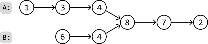
Output: Node 8
Intuitsiya
Avval ikki bog'liq ro'yxat orasidagi kesishma nima ekanligini tushunib olaylik.
Kesishma ikki bog'liq ro'yxat umumiy tugunga qo'shilganda va o'sha nuqtadan keyin ular bitta zanjir bo'lib qolganda yuzaga keladi.
E'tibor bering, ushbu kesishma tugunlarning qiymatlari bilan hech qanday aloqasi yo'q.
Sodda yondashuv hash to'plamdan foydalanishdir. Birinchi bog'liq ro'yxatni bir marta kesib o'tib har bir tugunni saqlashimiz mumkin va keyin ikkinchi bog'liq ro'yxatni kesib o'tganda bu to'plamni tekshirishimiz mumkin.
Quyidagi misolni ko'rib chiqing:
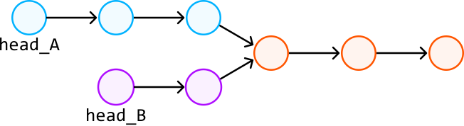
Bularni ikki alohida bog'liq ro'yxat sifatida ko'rib chiqish yuqoridagi vizualizatsiya bilan chalkashib ketishi mumkin. Buning o'rniga, ularni birlashtirilgan bog'liq ro'yxatlar sifatida ko'raylik.
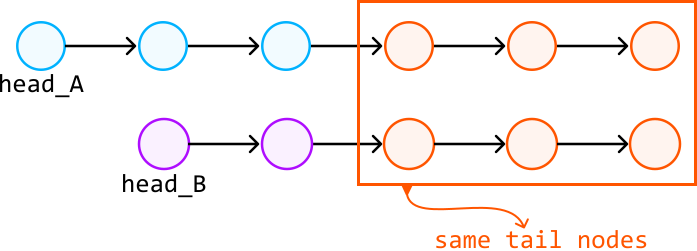
E'tibor bering, agar ikki bog'liq ro'yxat teng uzunlikda bo'lsa, masalani hal qilish osonroq bo'ladi. Buning sababi, teng uzunlikdagi bog'liq ro'yxatlar uchun o'sha indeksdagi tugunlarni taqqoslab kesishma tugunini topishimiz mumkin.
Turli uzunlikdagi bog'liq ro'yxatlar bilan ishlashda bu xatti-harakatni qandaydir tarzda takrorlay olamizmi? Asosiy tushuncha shundan iboratki, kesishuvdan keyingi qism ikki bog'liq ro'yxat uchun bir xil uzunlikka ega.
Endi biz bir xil uzunlikka ega bo'lgan, bir xil kesishmani bo'lishuvchi ikkita birlashtirilgan bog'liq ro'yxatni o'rnatdik.
Buni amalga oshirish uchun ikkala birlashtirilgan bog'liq ro'yxatni ikkita ko'rsatkich bilan kesib o'tib, ko'rsatkichlardagi tugunlar mos kelguncha to'xtatishimiz mumkin.
Agar kesishma mavjud bo'lmasa, ikki ko'rsatkich ham null tugunlarda to'xtaydi:
Birlashtirilgan bog'liq ro'yxatlar bo'ylab kesib o'tish Muhim kuzatuv shundan iboratki, 'A ro'yxati → B ro'yxati' orqali kesib o'tish uchun A ro'yxatining oxiriga yetganimizda B boshiga o'tishimiz kerak.
Bu texnika ikkala bog'liq ro'yxatning butun ketma-ketligini ulangan kabi kesib o'tish imkonini beradi.
Amalga oshirish
from ds import ListNode

def linked_list_intersection(head_A: ListNode, head_B: ListNode) -> ListNode:
    ptr_A, ptr_B = head_A, head_B
    # Traverse through list A with 'ptr_A' and list B with 'ptr_B' until they meet.
    while ptr_A != ptr_B:
        # Traverse list A -> list B by first traversing 'ptr_A' and then, upon
        # reaching the end of list A, continue the traversal from the head of list B.
        ptr_A = ptr_A.next if ptr_A else head_B
        # Simultaneously, traverse list B -> list A.
        ptr_B = ptr_B.next if ptr_B else head_A
    # At this point, 'ptr_A' and 'ptr_B' either point to the intersection node or both
    # are null if the lists do not intersect. Return either pointer.
    return ptr_A
Murakkablik Tahlili
Vaqt murakkabligi: linked_list_intersection ning vaqt murakkabligi O(n+m), bu yerda n va m ikkita bog'liq ro'yxatning uzunliklarini bildiradi.
Xotira murakkabligi: Xotira murakkabligi O(1).
LRU Kesh
LRU Kesh
Eng kam ishlatilgan (Least Recently Used — LRU) kesh uchun quyidagi operatsiyalarni qo'llab-quvvatlovchi ma'lumotlar strukturasini loyihalang va amalga oshiring:
- LRUCache(capacity: int): Belgilangan sig'imli LRU keshini ishga tushiring.
- get(key: int) -> int: Kalit bilan bog'liq qiymatni qaytaring. Kalit mavjud bo'lmasa -1 qaytaring.
- put(key: int, value: int) -> None: Keshga kalit va uning qiymatini qo'shing. Kalitni qo'shish keshning sig'imidan oshib ketishiga olib kelsa, eng kam ishlatilgan kalitni o'chiring.
Misol:
Input: [
  put(1, 100),
  put(2, 250),
  get(2),
  put(4, 300),
  put(3, 200),
  get(4),
  get(1),
],
  capacity = 3
Output: [250, 300, -1]
Tushuntirish:
put(1, 100)  # cache is[1: 100]
put(2, 250)  # cache is[1: 100, 2: 250]
get(2)       # return 250
put(4, 300)  # cache is[1: 100, 2: 250, 4: 300]t
put(3, 200)  # cache is[2: 250, 4: 300, 3: 200]
get(4)       # return 300
get(1)       # key 1 was evicted when adding key 3 due to the capacity
             # limit: return -1
Cheklovlar:
- Barcha kalitlar va qiymatlar musbat butun sonlar.
- Kesh sig'imi musbat.
Intuitsiya
Loyihalash masalasi bilan tanishganda, odatda birinchi qadamlar masalani tushunish va kerakli funktsiyalarni aniqlashdir.
Quyida ko'rsatilgan LRU keshini ko'rib chiqing. U hozirda 3 ta elementni o'z ichiga oladi va to'liq sig'imga yetdi.
Keshga yangi kalit-qiymat juftini kiritishga harakat qilaylik:
Bu yangi juft keshda eng yangi bo'ladi, shuning uchun u eng ko'p ishlatilgan uchda qo'shilishi kerak.
Ushbu umumiy ko'rinishdan put funksiyasini amalga oshirish uchun kerakli operatsiyalarni xulosalaymiz:
- Keshning eng kam ishlatilgan uchidan kalit-qiymat juftini olib tashlang.
- Keshning eng ko'p ishlatilgan uchiga kalit-qiymat juftini qo'shing.
Endi ushbu misol keshdan qiymatni olishga harakat qilaylik. get(2) bajarmasak, u 2 ning qiymatini qaytarishini kutamiz.

Bu misoldan get funksiyasi uchun ikkita asosiy amal aniqladik:
- Kalit-qiymat juftini keshning eng yangi uchiga ko'chiring.
- Kalit yordamida qiymatga kiring.
Loyihalashni yuqorida ko'rsatilgan to'rtta asosiy amalga qisqartirdik. Bular mos ma'lumotlar strukturalarini aniqlashga yordam beradi.
Ma'lumotlar strukturalarini tanlash Amallar 1 va 2
Birinchi ikki amal kalit-qiymat juftlarini qo'shish va o'chirishni o'z ichiga oladi. Xususan, keshning ixtiyoriy uchiga samarali kiritish va o'chirish imkoniyatimiz bo'lishi kerak.
Qaysi ma'lumotlar strukturasi elementni samarali qo'shish yoki olib tashlash imkonini beradi? Mos ma'lumotlar strukturasi — bog'liq ro'yxat, chunki u bosh yoki dumiga O(1) da qo'shish va o'chirish imkonini beradi.
Bir yo'nalishli va ikki yo'nalishli bog'liq ro'yxat
Bog'liq ro'yxatning boshidan tugunni qo'shish yoki olib tashlash O(1) vaqt oladi, u bir yo'nalishli yoki ikki yo'nalishli bo'lishidan qat'i nazar.
Bizga kerakli muhim xususiyat — kalit-qiymat juftlarini qo'shish va o'chirish paytida ikki yo'nalishli bog'liq ro'yxatning ikki uchiga ham kirish imkoniyati.
- Bog'liq ro'yxatning dumi eng ko'p ishlatilgan tugunni bildiradi.
- Bog'liq ro'yxatning boshi eng kam ishlatilgan tugunni bildiradi.
Bog'liq ro'yxatning uchlariga murojaat qilish uchun bosh va dum tugunlarini yaratishimiz mumkin, bu yerda bosh eng kam ishlatilgan tugunga va dum eng ko'p ishlatilgan tugunga ishora qiladi.

Amallar 3 va 4
3-amal tugunni bog'liq ro'yxatning eng ko'p ishlatilgan uchiga ko'chirish imkoniga ega bo'lishimiz kerakligini bildiradi. Bu O(1) da amalga oshirilishi uchun hash xaritaga bog'liq bo'ladi.

Hash xaritadan foydalanish kalitlardan qiymatlarni samarali qidirish bo'yicha 4-amalni ham hal qiladi.
LRU keshini ifodalash uchun ikki yo'nalishli bog'liq ro'yxat va hash xaritadan foydalanishga qaror qildik, endi asosiy operatsiyalarni ko'rib chiqaylik.
put(key: int, val: int) -> None: Quyida keshga yangi kalit-qiymat juftini qo'shish uchun oqim ko'rsatilgan.
To'liq sig'imga yetgan ikki yo'nalishli bog'liq ro'yxatga yangi tugunni qanday qo'shishni yaxshiroq tushunish uchun tekshiring.
Ko'rib turganingizdek, bizga tugunni olib tashlash funksiyasi (remove_node) hamda dum qismiga tugun qo'shish funksiyasi (add_tail_node) kerak bo'ladi.
get(key: int) -> int: Quyida keshdan kalitning qiymatini olish jarayoni ko'rsatilgan:
Endi get funksiyasi chaqiruvi davomida ikki yo'nalishli bog'liq ro'yxat qanday yangilanishini ko'rib chiqaylik.
![Image represents a visual depiction of a `get(2)` operation on a doubly linked list, implemented using a hashmap for efficient node access. The top section shows the initial state: a doubly linked list with nodes labeled '2 | 250', '4 | 300', and '3 | 200', connected by bidirectional arrows indicating `next` and `prev` pointers. 'head' and 'tail' labels point to the beginning and end of the list, respectively. A dashed arrow points from `remove_node(hashmap[2])` to node '2 | 250', which is marked with a red 'X', signifying its removal. The middle section illustrates the removal of node '2 | 250'. The bottom section shows the node '2 | 250' re-added to the tail of the list via `add_to_tail(2 | 250)`, indicated by a dashed arrow. Finally, a thick black arrow at the bottom points to 'return 250', indicating the value returned by the `get(2)` operation after the node has been temporarily removed and then re-added to the tail. Each node displays a key-value pair (e.g., '2 | 250'), representing the key used in the hashmap and the associated value. The overall diagram demonstrates the process of retrieving a node's value, removing it, and then re-inserting it at the tail to maintain the list's structure.](https://bytebytego.com/images/courses/coding-patterns/linked-lists/lru-cache/image-03-04-12-JETT4CZS.svg?dpl=dpl_Gs7zfM6MUzjTBjcjps1LqXtb9QmD)
Endi ikki yo'nalishli bog'liq ro'yxat va hash xaritaning LRU keshini loyihalash uchun qanday ishlatilishini tushunganligi sababli, kodni ko'rib chiqaylik.
Amalga oshirish
Quyidagi maxsus sinfdan ikki yo'nalishli bog'liq ro'yxatdagi tugunni ifodalash uchun foydalanishimiz mumkin:
class DoublyLinkedListNode:
   def __init__(self, key: int, val: int):
       self.key = key
       self.val = val
       self.next = self.prev = None
Quyidagi misol bog'liq ro'yxatning dumiga tugunni qanday qo'shishni ko'rsatadi. Yangi tugunni new_node, undan oldingi tugunni esa prev_node deb ataymiz.
Yangi tugun prev_node dan keyin va dum tugunidan oldin ko'rinishi kerak. Yangi tugunning prev va next ni o'rnataylik.
Endi prev_node va dum tugunini yangi tugunga bog'lang:
Quyida ushbu funksiyaning amalga oshirilishi keltirilgan:
def add_to_tail(self, node: DoublyLinkedListNode) -> None:
    prev_node = self.tail.prev
    node.prev = prev_node
    node.next = self.tail
    prev_node.next = node
    self.tail.prev = node
Quyidagi misol ikki yo'nalishli bog'liq ro'yxatdan tugunni qanday olib tashlashni ko'rsatadi:
Tugunni olib tashlash uchun uning ikkita qo'shni tugunini bir-biriga ishora qildiramiz, samarali ravishda tugunni chiqarib tashlaymiz.

Quyida ushbu funksiyaning amalga oshirilishi keltirilgan:
def remove_node(self, node: DoublyLinkedListNode) -> None:
    node.prev.next = node.next
    node.next.prev = node.prev
Yuqoridagi ikkita funksiya yordamida LRU keshining to'liq amalga oshirilishini yakunlaymiz.
LRU Kesh
class DoublyLinkedListNode:
    def __init__(self, key: int, val: int):
        self.key = key
        self.val = val
        self.next = self.prev = None

class LRUCache:
    def __init__(self, capacity: int):
        self.capacity = capacity
        # A hash map that maps keys to nodes.
        self.hashmap = {}
        # Initialize the head and tail dummy nodes and connect them to
        # each other to establish a basic two-node doubly linked list.
        self.head = DoublyLinkedListNode(-1, -1)
        self.tail = DoublyLinkedListNode(-1, -1)
        self.head.next = self.tail
        self.tail.prev = self.head

    def get(self, key: int) -> int:
        if key not in self.hashmap:
            return -1
        # To make this key the most recently used, remove its node and
        # re-add it to the tail of the linked list.
        self.remove_node(self.hashmap[key])
        self.add_to_tail(self.hashmap[key])
        return self.hashmap[key].val

    def put(self, key: int, value: int) -> None:
        # If a node with this key already exists, remove it from the
        # linked list.
        if key in self.hashmap:
            self.remove_node(self.hashmap[key])
        node = DoublyLinkedListNode(key, value)
        self.hashmap[key] = node
        # Remove the least recently used node from the cache if adding
        # this new node will result in an overflow.
        if len(self.hashmap) > self.capacity:
            del self.hashmap[self.head.next.key]
            self.remove_node(self.head.next)
        self.add_to_tail(node)

    def add_to_tail(self, node: DoublyLinkedListNode) -> None:
        prev_node = self.tail.prev
        node.prev = prev_node
        node.next = self.tail
        prev_node.next = node
        self.tail.prev = node

    def remove_node(self, node: DoublyLinkedListNode) -> None:
        node.prev.next = node.next
        node.next.prev = node.prev
Murakkablik Tahlili
Vaqt murakkabligi: remove_node va add_tail_node yordamchi funksiyalarining vaqt murakkabligi O(1). Shuning uchun get va put funksiyalarining vaqt murakkabligi ham O(1).
Xotira murakkabligi: Ushbu yechimning umumiy xotira murakkabligi O(n), bu yerda n kesh sig'imidir.
Intervyu Maslahat
Maslahat: Ma'lumotlar strukturalarini birlashtirish ma'lum funktsiyalarni qanday ta'minlash mumkinligini o'rganing. Ma'lum operatsiyalarni samarali bajara oluvchi ma'lumotlar strukturasini amalga oshirish uchun bir nechta ma'lumotlar strukturalarini birlashtirish mumkin.
Palindromik Bog'liq Ro'yxat
Palindromik Bog'liq Ro'yxat
Bir yo'nalishli bog'liq ro'yxatning boshi berilgan, u palindrom ekanligini aniqlang.
Misol 1:

Output: True
Misol 2:

Output: False
Intuitsiya
Agar bog'liq ro'yxat qiymatlari oldinga ham, orqaga ham bir xil o'qilsa, u palindromikdir. Sodda usul — bog'liq ro'yxat qiymatlarini massivda saqlash va palindrom ekanligini massivdan tekshirishdir.
Yuqoridagi ta'rifdan kelib chiqib, agar bog'liq ro'yxat palindrom bo'lsa, uni teskari aylantirish bir xil qiymatlarga olib kelishini bilamiz.
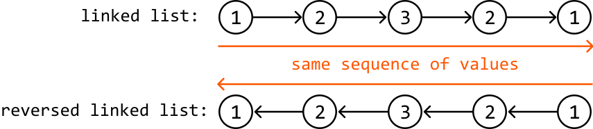
Bu shuni anglatadiki, bog'liq ro'yxatning nusxasini yaratib, uni teskari aylantirish va asl ro'yxat bilan qiymatlarini taqqoslashimiz mumkin edi.
Muhim kuzatuv shundan iboratki, biz faqat asl bog'liq ro'yxatning birinchi yarmini teskari aylantirilgan ikkinchi yarmi bilan taqqoslashimiz kerak.
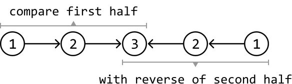
Bu taqqoslashni amalga oshirishdan oldin quyidagilarni bajarishimiz kerak:
- Ikkinchi yarmining boshini olish uchun bog'liq ro'yxatning o'rtasini toping.
- Ushbu o'rta tugundan boshlab bog'liq ro'yxatning ikkinchi yarmini teskari aylantiring.
E'tibor bering, 2-qadam kiritilgan ma'lumotni o'zgartirishni o'z ichiga oladi. Bu masalada buni qabul qilish mumkin deb faraz qilaylik.
Endi bu ikki qadam qanday qo'llanilishini ko'rib chiqaylik. Bog'liq ro'yxatning o'rta tugunini (mid) topishdan boshlang.
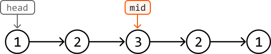
Bog'liq ro'yxatning o'rtasiga qanday yetishni o'rganish uchun Bog'liq Ro'yxat O'rta Nuqtasi tushuntirishini o'qing.
Keyin, mid dan boshlab bog'liq ro'yxatning ikkinchi yarmini teskari aylantiring. Asl bog'liq ro'yxatning oxirgi tuguni yangi bosh bo'ladi.

Bog'liq ro'yxatni O(n) vaqtda qanday teskari aylantirish haqida o'rganish uchun Bog'liq Ro'yxatni Teskari Aylantirish tushuntirishini o'qing.
Oxirgi qilishimiz kerak bo'lgan narsa — birinchi yarmining endi teskari aylantirilgan ikkinchi yarmi bilan mos kelishini tekshirishdir.
Bog'liq ro'yxatning birinchi va teskari aylantirilgan ikkinchi yarmlari bo'ylab takrorlash uchun ikkita ko'rsatkich (ptr1 va ptr2) dan foydalanishimiz mumkin.
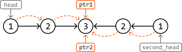
Amalga oshirish
from ds import ListNode

def palindromic_linked_list(head: ListNode) -> bool:
    # Find the middle of the linked list and then reverse the second half of the # linked list starting at this midpoint.
    mid = find_middle(head)
    second_head = reverse_list(mid)
    # Compare the first half and the reversed second half of the list
    ptr1, ptr2 = head, second_head
    res = True
    while ptr2:
        if ptr1.val != ptr2.val:
            res = False
        ptr1, ptr2 = ptr1.next, ptr2.next
    return res

# From the 'Reverse Linked List' problem.
def reverse_list(head: ListNode) -> ListNode:
    prevNode, currNode = None, head
    while currNode:
        nextNode = currNode.next
        currNode.next = prevNode
        prevNode = currNode
        currNode = nextNode
    return prevNode

# From the 'Linked List Midpoint' problem.
def find_middle(head: ListNode) -> ListNode:
    slow = fast = head
    while fast and fast.next:
        slow = slow.next
        fast = fast.next.next
    return slow
Murakkablik Tahlili
Vaqt murakkabligi: palindromic_linked_list ning vaqt murakkabligi O(n), bu yerda n bog'liq ro'yxatdagi tugunlar sonini bildiradi.
Xotira murakkabligi: Xotira murakkabligi O(1).
Intervyu Maslahat
Maslahat: Bog'liq ro'yxatni o'zgartirish maqbulmi, aniqlang. Yechimimizda ikkinchi yarmini teskari aylandirdik, bu kiritilgan bog'liq ro'yxatni o'zgartiradi.
Ko'p Darajali Bog'liq Ro'yxatni Yassilash
Ko'p Darajali Bog'liq Ro'yxatni Yassilash
Ko'p darajali bog'liq ro'yxatda har bir tugunning keyingi ko'rsatkichi va bola ko'rsatkichi bor. Keyingi ko'rsatkich bir xil darajadagi keyingi tugunga ishora qiladi, bola ko'rsatkichi esa quyi darajadagi bog'liq ro'yxatga ishora qilishi mumkin.
Ko'p darajali bog'liq ro'yxatni har bir darajaning oxirini keyingi darajaning boshiga ulash orqali yagona darajali bog'liq ro'yxatga tekislashtiring.
Misol:
Intuitsiya
Yassilangan bog'liq ro'yxatni hosil qilish uchun zarur bo'lgan ikkita asosiy shartni ko'rib chiqing:
- Har bir darajadagi tugunlarning tartibi saqlanishi kerak.
- Bir darajadagi barcha tugunlar keyingi darajadagi tugunlarni qo'shishdan oldin ulangan bo'lishi kerak.
Bu masalaning qiyinligi — quyi darajalardagi bog'liq ro'yxatlarni qanday qayta ishlashni aniqlashdir. Bir strategiya — har bir darajani alohida qayta ishlashdir.
Asosiy kuzatuv shundan iboratki, ko'p darajali bog'liq ro'yxatning ixtiyoriy 'L' darajasi uchun, biz 'L' darajasidagi barcha tugunlarga to'g'ridan-to'g'ri kirishimiz bor.
'L + 1' darajasidagi tugunlarni 'L' darajasining oxiriga qanday ulashimiz mumkin? Biz 'L' darajasidagi joriy tugundan keyingi ko'rsatkich orqali 'L' darajasining dumiga ega bo'lganligi sababli, 'L' darajasining dumini 'L + 1' darajasining boshiga ulashimiz mumkin.
Shunday qilib, 'L + 1' darajasidagi barcha tugunlar 'L' darajasiga qo'shilgandan so'ng, 'L + 2' darajasini 'L + 1' darajasiga qo'shish jarayonini davom ettirishimiz mumkin.
Yuqori darajadagi g'oya haqida fikrimiz borligidan, quyidagi misol bo'yicha ushbu strategiyani sinab ko'raylik.
2-darajaning tugunlarini 1-darajaning oxiriga qo'shishdan boshlaymiz. Buni amalga oshirishdan oldin 1-darajadagi dum tugunini topishimiz kerak.

Endi bola bog'liq ro'yxatlarini (5 → 6 va 7 → 8) dum tuguniga qo'shamiz. Dum ko'rsatkichini 1-darajadagi barcha tugunlar qo'shilguncha birga saqlaymiz.
Ushbu bola bog'liq ro'yxatini dum tugunining oxiriga qo'shish uchun tail.next ni bola bog'liq ro'yxatining boshiga o'rnating.


Bola ko'rsatkichiga ega keyingi tugunni topish uchun curr ni oshirishdan oldin dum ko'rsatkichini qayta sozlashimiz kerak.

Dum ko'rsatkichi qayta joylashtirilgandan so'ng, quyidagi jarayonni davom ettirishimiz mumkin:
- curr ko'rsatkichi yordamida bola bog'liq ro'yxatiga ega keyingi tugunni topish.
- Bola bog'liq ro'yxatini dum tuguniga qo'shish.
- Dum ko'rsatkichini yassilangan bog'liq ro'yxatning oxirgi tuguniga siljitish.


Jarayon tugagandan so'ng, yassilangan bog'liq ro'yxatning boshi bo'lgan head ni qaytarishimiz mumkin.
Oxirgi muhim tafsilot — ixtiyoriy bola bog'liq ro'yxatini dumga qo'shganidan so'ng, joriy tugunning bola ko'rsatkichini null ga o'rnatishimiz kerak.
Amalga oshirish
MultiLevelListNode sinfining ta'rifi quyida keltirilgan:
class MultiLevelListNode:
    def __init__(self, val, next, child):
        self.val = val
        self.next = next
        self.child = child
from ds import MultiLevelListNode

def flatten_multi_level_list(head: MultiLevelListNode) -> MultiLevelListNode:
    if not head:
        return None
    tail = head
    # Find the tail of the linked list at the first level.
    while tail.next:
        tail = tail.next
    curr = head
    # Process each node at the current level. If a node has a child linked list,
    # append it to the tail and then update the tail to the end of the extended linked
    # list. Continue until all nodes at the current level are processed.
    while curr:
        if curr.child:
            tail.next = curr.child
            curr.child = None
            while tail.next:
                tail = tail.next
        curr = curr.next
    return head
Murakkablik Tahlili
Vaqt murakkabligi: flatten_multi_level_list ning vaqt murakkabligi O(n), bu yerda n bog'liq ro'yxatdagi barcha darajalardagi tugunlarning umumiy sonini bildiradi.
Xotira murakkabligi: Biz faqat doimiy sondagi o'zgaruvchilar ajratdik, shuning uchun xotira murakkabligi O(1).
Tez va Sekin Ko'rsatkichlar
Tez va Sekin Ko'rsatkichlarga Kirish
Tez va Sekin Ko'rsatkichlarga Kirish
Intuitsiya
Tez va sekin ko'rsatkich texnikasi — ikki ko'rsatkich namunasining ixtisoslashgan varianti bo'lib, ikki ko'rsatkich turli tezliklarida harakatlanishi bilan tavsiflanadi.
- Odatda sekin ko'rsatkich har iteratsiyada bir qadam siljiydi.
- Odatda tez ko'rsatkich har iteratsiyada ikki qadam siljiydi.
Bu tez ko'rsatkich sekin ko'rsatkichdan ikki baravar tezroq harakatlanadigan dinamika yaratadi:
Esda tuting, bu ko'rsatkichlar faqat bir va ikki qadamga cheklanmagan. Tez ko'rsatkich sekin ko'rsatkichdan ko'proq qadam siljigani sari, siz ushbu texnikani tez va sekin ko'rsatkichlar namunasiga ega deb atashingiz mumkin.
Hayotiy Misol
Simlink lar dagi tsikllarni aniqlash: Simlink lar fayl tizimidagi fayl yoki kataloglarga ishora qiladigan yorliqlar. Tsiklli simlink — o'ziga yoki ajdodiga ishora qiladigan simlink.
Ushbu jarayonda sekin ko'rsatkich har bir simlink ni bir qadam siljitsa, tez ko'rsatkich ikkita simlink ni siljitadi. Agar ular uchrashuv qilsa, tsikl aniqlangan.
Bob Mazmuni
Tez va sekin ko'rsatkichlar indeks asosidagi kirishni qo'llab-quvvatlamaydigan bog'liq ro'yxatlar kabi ma'lumotlar strukturalarida ayniqsa foydali.
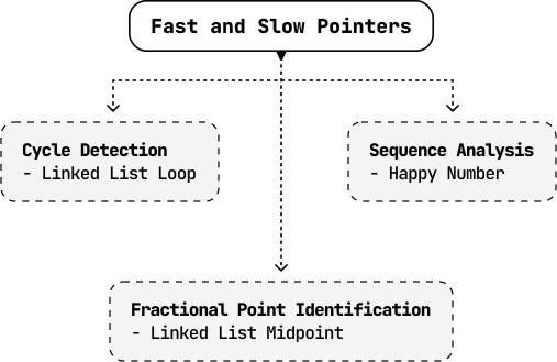
Bog'liq Ro'yxat Halqasi
Bog'liq Ro'yxat Halqasi
Bir yo'nalishli bog'liq ro'yxat berilgan, unda tsikl borligini aniqlang. Tugunning keyingi ko'rsatkichi ro'yxatdagi avvalgi tugunga ishora qilsa, tsikl yuzaga keladi.
Misol:
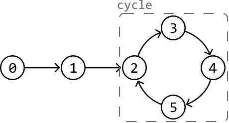
Output: True
Intuitsiya
Sodda yondashuv — allaqachon ko'rilgan tugunlarni kuzatib borib bog'liq ro'yxatni ko'rib chiqishdir.
from ds import ListNode

def linked_list_loop_naive(head: ListNode) -> bool:
    visited = set()
    curr = head
    while curr:
        # Cycle detected if the current node has already been visited.
        if curr in visited:
            return True
        visited.add(curr)
        curr = curr.next
    return False
Bu yechim O(n) vaqt oladi, bu yerda n bog'liq ro'yxatdagi tugunlar soni, chunki har bir tugun bir marta ko'riladi. Biroq, hash to'plam uchun O(n) qo'shimcha xotira talab qiladi.
Doira treklarni doiraviy bog'liq ro'yxat (ya'ni mukammal tsiklli bog'liq ro'yxat) sifatida tasavvur qiling, unda sekin va tez yugurmchi sifatida ko'rsatilgan ikkita yuguruvchi bor.
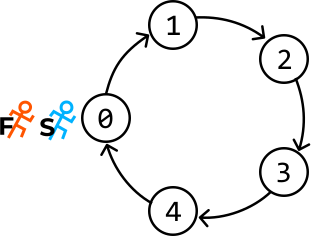
Agar ikki yuguruvchi bir xil tezlikda harakat qilsa, har bir tugunga birgalikda keladi. Biroq, bir yuguruvchi ikkinchisidan ikki baravar tezroq harakat qilsa nima bo'lishini ko'rib chiqing.
Bog'liq ro'yxatda tez yuguruvchi sekin yuguruvchidan o'tib ketganini aniqlash qiyin, chunki indeks asosidagi kirish mavjud emas.
Endi savol shuki, tez yuguruvchi sekin yuguruvchi bilan qayta uchrashadi, yoki tez yuguruvchi sekin yuguruvchidan cheksiz o'tib ketishi mumkinmi?
Mukammal tsikl Avval sekin va tez ko'rsatkich sifatida ifodalangan ikki yuguruvchi tsiklli bog'liq ro'yxatda uchrashib-uchrashmasligini tekshiraylik.
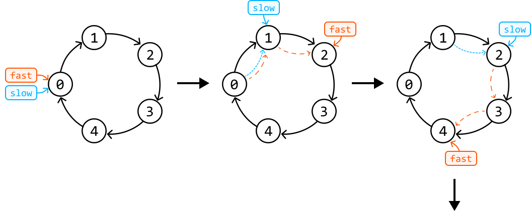
Kechiktirilgan tsikl Bog'liq ro'yxatda tsikl darhol boshlanmasa nima bo'ladi? Tez va sekin ko'rsatkichlar tsiklga turli nuqtalardan kirganida simulyatsiyani ko'rib chiqing.
Yana, tez va sekin tsiklga turli nuqtalardan kirganiga qaramay ko'rsatkichlar nihoyat tsikl ichida uchrashdi.
Tez ko'rsatkich har doim sekin ko'rsatkichga yetib oladimi? Ikkala holatda ham tez ko'rsatkich sekin ko'rsatkichni doimo o'tkazib yuborib turishi mumkin dek ko'rinishi mumkin.
Tez ko'rsatkich bir vaqtda 2 qadam, sekin ko'rsatkich 1 qadam siljiganligi sababli, tez ko'rsatkich sekin ko'rsatkichga har iteratsiyada 1 qadam yaqinlashadi.
Shuning uchun tez ko'rsatkich sekin ko'rsatkichga yetib olishi uchun kerakli maksimal qadamlar soni k bo'lib, bu yerda k ular o'rtasidagi masofa.
Tsikl yo'q So'nggi holat — tsikl yo'q. Bu holatda tez ko'rsatkich nihoyat bog'liq ro'yxat oxiriga yetib, null ga tushadi.
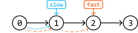

Amalga oshirish
Ushbu algoritm rasmiy ravishda 'Floyd ning Tsikl Aniqlash' algoritmi [1] deb nomlanadi.
from ds import ListNode

def linked_list_loop(head: ListNode) -> bool:
    slow = fast = head
    # Check both 'fast' and 'fast.next' to avoid null pointer exceptions when we
    # perform 'fast.next' and 'fast.next.next'.
    while fast and fast.next:
        slow = slow.next
        fast = fast.next.next
        if fast == slow:
            return True
    return False
Murakkablik Tahlili
Vaqt murakkabligi: linked_list_loop ning vaqt murakkabligi O(n), chunki tez ko'rsatkich bog'liq ro'yxatni ko'pi bilan ikki marta ko'rib chiqgandan so'ng sekin ko'rsatkich bilan uchrashuv qiladi.
Xotira murakkabligi: Xotira murakkabligi O(1).
Bog'liq Ro'yxatning O'rta Nuqtasi
Bog'liq Ro'yxatning O'rta Nuqtasi
Bir yo'nalishli bog'liq ro'yxat berilgan, uning o'rta tugunini toping va qaytaring. Ikkita o'rta tugun mavjud bo'lsa, ikkinchisini qaytaring.
Misol 1:

Output: Node 4
Misol 2:

Output: Node 4
Cheklovlar:
- Bog'liq ro'yxat kamida bitta tugunni o'z ichiga oladi.
- Bog'liq ro'yxat noyob qiymatlarni o'z ichiga oladi.
Intuitsiya
Bu masalani hal qilishning eng intuitiv yondashuvi — bog'liq ro'yxatni uzunligini (n) topish uchun kesib o'tish va keyin yana n/2 tugunga o'tishdir.
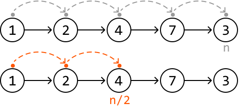
Bu yondashuv O(n) vaqtda masalani hal qiladi, lekin o'rta nuqtani topish uchun ikki iteratsiyani talab qiladi. Biroq, biz buni bitta o'tishda amalga oshira olamizmi?
Bog'liq ro'yxatni ko'rib chiqayotganda, aniq pozitsiyamiz noma'lum. Faqat oxirga yetganimizda qaerdajamligi bilamiz.
Agar bitta ko'rsatkich boshqasidan ikki baravar sekin harakat qilsa, tez ko'rsatkich oxirga yetganida sekin ko'rsatkich o'rtada bo'ladi.
Buni tez va sekin ko'rsatkich texnikasidan foydalanib amalga oshirishimiz mumkin:
- Sekin ko'rsatkichni bir vaqtda bir tugunga siljiting.
- Tez ko'rsatkichni bir vaqtda ikki tugunga siljiting.
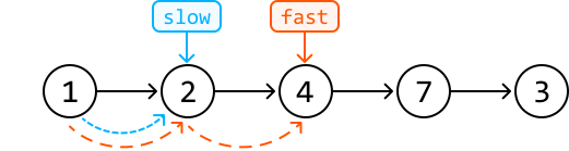

E'tibor berishimiz kerak bo'lgan narsa — tez ko'rsatkichni qachon to'xtatishimiz kerak. Tez ko'rsatkich bog'liq ro'yxatdan tashqariga chiqib ketmaslik uchun to'xtatishimiz kerak.
Bog'liq ro'yxat uzunligi juft bo'lganda nima bo'ladi? Quyidagi misolni ko'rib chiqing:
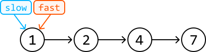
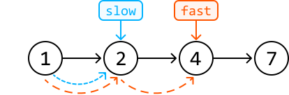

Ko'rib turganingizdek, sekin ikkinchi o'rta tugunga ishora qilishi uchun tez null tugunga yetganda to'xtatishimiz kerak.
Amalga oshirish
from ds import ListNode

def linked_list_midpoint(head: ListNode) -> ListNode:
    slow = fast = head
    # When the fast pointer reaches the end of the list, the slow pointer will be at
    # the midpoint of the linked list.
    while fast and fast.next:
        slow = slow.next
        fast = fast.next.next
    return slow
Murakkablik Tahlili
Vaqt murakkabligi: linked_list_midpoint ning vaqt murakkabligi O(n), chunki biz bog'liq ro'yxatni tezkor ko'rsatkich yordamida to'liq kesib o'tamiz.
Xotira murakkabligi: Xotira murakkabligi O(1).
To'xtab O'ylang
Agar bog'liq ro'yxat juft uzunlikda bo'lganda birinchi o'rta tugunni qaytarish uchun algoritmingizni o'zgartirishingizni so'rashsa?
Javob: Bir xil usulni qo'llab, fast.next.next null bo'lganda tez ko'rsatkichni oldinga siljitishni to'xtatishimiz kerak. Bu sekin ko'rsatkichni birinchi o'rta tugunga to'xtatadi.

Intervyu Maslahat
Maslahat: Berilgan ma'lumotlardagi potentsial bo'shliqlarni ko'rib chiqishga tayyor bo'ling. Intervyu davomida intervyu olib boruvchi cheklovlarni to'liq belgilamasligi mumkin.
Baxtli Son
Baxtli Son
Son nazariyasida baxtli son — har bir xonasini kvadratga ko'tarish va natijalarni qo'shish jarayoni takrorlanganida oxir-oqibat 1 ga olib keladigan son.
Butun son berilgan, u baxtli son ekanligini aniqlang.
Misol:
Input: n = 23
Output: True
Tushuntirish: 2² + 3² = 13 ⇒ 1² + 3² = 10 ⇒ 1² + 0² = 1
Intuitsiya
Har bir xonaning kvadratlarini qo'shib takrorlash jarayonini simulyatsiya qilib baxtli sonni aniqlay olamiz.
Masala ta'rifiga ko'ra, bu jarayon ikki yo'ldan biri bilan tugashi mumkin:
- 1-holat: jarayon yakuniy son 1 bo'lgunga qadar davom etadi.
- 2-holat: jarayon cheksiz siklga tushib qoladi.
Ikkala ssenariyni diagramma qilsak, qiziqarli narsa ko'ramiz:
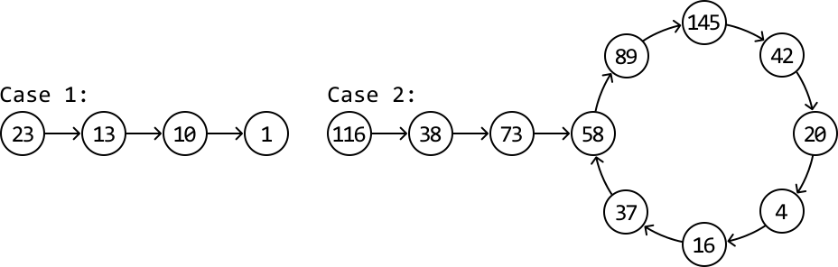
Bu bog'liq ro'yxat masalasiga juda o'xshaydi. Xususan, bog'liq ro'yxatda tsikl borligini aniqlash masalasi.
Bu masalani Bog'liq Ro'yxat Halqasi masalidagi kabi tsikl aniqlash muammosiga qisqartirishimiz mumkin. Tez va sekin ko'rsatkich algoritmini qo'llab, biz sonlar ketma-ketligidagi tsikllarni aniqlay olamiz.
Biroq, bu masalada tez va sekin ko'rsatkich algoritmini bajarish uchun haqiqiy bog'liq ro'yxatimiz yo'q.
Qulay tomoni shuki, ixtiyoriy x son uchun ketma-ketlikdagi 'keyingi' son nima ekanini allaqachon bilamiz. Masala ta'rifida aytilganidek, keyingi son x ning har bir xonasi kvadratlarining yig'indisidir.
Ketma-ketlikdagi keyingi sonni olish x ning keyingi sonini hisoblash uchun uning har bir xonasiga kirishning usuli kerak.
- Modulo operatsiyasi (x % 10) x sonining oxirgi xonasini ajratib olish uchun ishlatiladi.
- x ni 10 ga bo'ling (x = x / 10) va oxirgi xonani kesib tashlang, keyingi xona yangi oxirgi xonaga o'tadi.
x = 123 uchun bu jarayon quyida to'liq ko'rsatilgan:
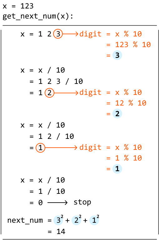
Ketma-ketlikni kesib o'tish usulimiz borligiga ko'ra, Floyd ning Tsikl Aniqlash algoritmini amalga oshirishimiz mumkin. Boshlash uchun:
- Sekin ko'rsatkichni bir vaqtda bitta son siljiting (slow = get_next_num(slow)).
- Tez ko'rsatkichni bir vaqtda ikkita son siljiting (fast = get_next_num(get_next_num(fast))).
Agar jarayon davomida tez va sekin ko'rsatkichlar uchrashuv qilsa, bu tsikl mavjudligini ko'rsatadi, ya'ni son baxtli emas.
Amalga oshirish
def happy_number(n: int) -> bool:
    slow = fast = n
    while True:
        slow = get_next_num(slow)
        fast = get_next_num(get_next_num(fast))
        if fast == 1:
            return True
        # If the fast and slow pointers meet, a cycle is detected. Hence, 'n' is not
        # a happy number.
        elif fast == slow:
            return False

def get_next_num(x: int) -> int:
    next_num = 0
    while x > 0:
        # Extract the last digit of 'x'.
        digit = x % 10
        # Truncate (remove) the last digit from 'x' using floor division.
        x //= 10
        # Add the square of the extracted digit to the sum.
        next_num += digit ** 2
    return next_num
Murakkablik Tahlili
Vaqt murakkabligi: happy_number ning vaqt murakkabligi O(log(n)). Buning to'liq tahlili ushbu qismda muhokama qilingan.
Xotira murakkabligi: Xotira murakkabligi O(1).
Intervyu Maslahat
Maslahat: Masalani vizuallang. Birinchi qarashda bu masala matematik fikrlashni talab qiladigan ko'rinishi mumkin.
Baxtli Son Vaqt Murakkabligi Tahlili
Quyidagi vaqt murakkabligi tahlili baxtli sonni aniqlash uchun kerakli qadamlarda yuqori chegarani belgilaydi.
1) Keyingi son uchun yuqori chegara Belgilangan xonalar soniga ega ixtiyoriy n son uchun, keyingi sonining maksimal qiymati.
2) Xonalar soniga nisbatan keyingi sonning hajmi
- Agar n son 1 yoki 2 xonali bo'lsa, keyingi son n dan katta bo'lishi mumkin (masalan, keyingi son uchun).
- Agar n son 3 yoki undan ko'p xonali bo'lsa, keyingi son har doim n ning asl qiymatidan kichik bo'ladi.
| Digits | Largest Number | Next Number |
|---|---|---|
| 1 | 9 | 81 |
| 2 | 99 | 162 |
| 3 | 999 | 243 |
| 4 | 9999 | 324 |
| 5 | 99999 | 405 |
| 6 | 999999 | 486 |
| ... | ... | ... |
3) Tsikllar uchun xulosalar Uch va undan ko'p xonali sonlar uchun keyingi son doimo kichikroq bo'lganligi sababli, oxir-oqibat 1 dan 243 gacha diapazon ichida son hosil bo'ladi.
4) 243 dan kichik sonlar uchun vaqt murakkabligi Son 243 dan past tushgandan so'ng, algoritm 1 ga yetish yoki tsiklga kirishdan oldin 243 dan kam qadamda bajariladi.
5) 243 dan katta sonlar uchun vaqt murakkabligi Sondagi xonalar soni taxminan log(n) ga teng.
n ning keyingi sonini n2 deb ataymiz. n2 dan keyingi son (n3) taxminan log(n2) = log(log(n)) qadamda bajariladi.
Xulosa n 243 dan kichik bo'lganda, vaqt murakkabligi O(1), n 243 dan katta bo'lganda esa vaqt murakkabligi O(log(n)).
Intervyu Maslahat
Maslahat: Agar intervyuning muhim qismi bo'lmasa, murakkab isbotlarga vaqt sarflamang.
Intervyu davomida ushbu masalani hal qilish uchun ishlatiladigan kabi algoritmning aniq vaqtini to'g'ri aniqlash uchun chuqur matematik tahlil talab qilinishi mumkin.
Siljuvchi Oynalar
Siljuvchi Oynalarga Kirish
Siljuvchi Oynalarga Kirish
Intuitsiya
Siljuvchi oyna texnikasi — ikki ko'rsatkich namunasining bir qismi bo'lib, ikkita ko'rsatkich (odatda chap va o'ng) yordamida ma'lumotlar strukturasidagi qo'shni quyi qismni aniqlaydi.
![The image represents a sliding window concept often used in algorithms. It shows a sequence of elements represented by dots enclosed in square brackets `[ . . . . . . ]`. A light-blue rectangular area highlights a subset of these elements, labeled 'window'. Two rectangular boxes, labeled 'left' and 'right,' are positioned above the sequence. A downward-pointing arrow connects 'left' to the leftmost dot within the window, and a similar arrow connects 'right' to the rightmost dot within the window. A light-blue upward-pointing arrow labeled 'window' indicates that this window can move along the sequence. The arrangement visually demonstrates how the window's position is controlled by the 'left' and 'right' pointers, allowing it to slide across the data sequence, processing a fixed-size subset at a time.](https://bytebytego.com/images/courses/coding-patterns/sliding-windows/introduction-to-sliding-windows/image-05-00-1-6W2RRYSN.svg?dpl=dpl_Gs7zfM6MUzjTBjcjps1LqXtb9QmD)
Siljuvchi oynalar, algoritm aks holda ikkita ichki tsiklga taylanadigan holatlarda ayniqsa qimmatlidir.
- Oynani kengaytirish — o'ng ko'rsatkichni oldinga siljitish:
- Oynani toraytirish — chap ko'rsatkichni oldinga siljitish:
- Oynani siljitish — chap va o'ng ko'rsatkichlarni ikkovini oldinga siljitish: E'tibor bering, siljitish kengaytirish va keyin toraytirishga teng.
Endi ikki asosiy turdagi siljuvchi oyna algoritmlarini ko'rib chiqaylik:
- Belgilangan siljuvchi oyna.
- Dinamik siljuvchi oyna.
Belgilangan Siljuvchi Oyna
Belgilangan siljuvchi oyna ma'lumotlar strukturasi bo'ylab siljiganda ma'lum uzunlikni saqlab qoladi.

Masala bizdan ma'lum uzunlikdagi quyi qismni topishni so'raganda belgilangan siljuvchi oyna texnikasini qo'llaymiz.
Agar k uzunligidagi belgilangan oyna ma'lumotlar strukturasini boshidan oxirigacha o'tsa, u k uzunlikdagi har bir quyi qismni ko'rishi kafolatlanadi.
Quyida belgilangan siljuvchi oynaning ma'lumotlar strukturasi bo'ylab qanday harakatlanishining umumiy shabloni keltirilgan.
left = right = 0
while right < n:
    # If the window has reached the expected fixed length, we slide the window (move
    # both left and right).
    if right - left + 1 == fixed_window_size:
        # Process the current window.
        result = process_current_window()
        left += 1
    right += 1
Dinamik Siljuvchi Oyna
Belgilangan siljuvchi oynalardan farqli o'laroq, dinamik oynalar ma'lumotlar strukturasi bo'ylab harakatlanayotganda kengayishi yoki torayishi mumkin.

Odatda, dinamik siljuvchi oynalar bizdan ma'lum shart asosida eng uzun yoki eng qisqa quyi qismni topishni so'raydigan masalalarga qo'llanilishi mumkin.
Eng uzun quyi qismni topishda kengaytirish va toraytirish dinamikasi odatda quyidagicha:
- Agar oyna shartni qondirsa, shartni ham qondiradigan uzunroq oyna topish uchun uni kengaytiring.
- Agar shart buzilsa, shart yana qondirilguncha oynani toraytiring.
Quyida bu qanday ishlashini ko'rsatuvchi umumiy shablon keltirilgan:
left = right = 0
while right < n:
    # While the condition is violated, the window is invalid, so shrink the window by
    # advancing the left pointer.
    while condition is violated:
        left += 1
    # Once the window is valid, process it and then expand the window by advancing the
    # right pointer.
    result = process_current_window()
    right += 1
E'tibor bering, belgilangan va dinamik oynalar uchun taqdim etilgan shablonlar asosan chap va o'ng ko'rsatkichlarning harakatini ta'kidlaydi.
Hayotiy Misol
Video oqimida buferlash: Video oqimida buferlashtirish va o'ynash sifatini boshqarish uchun dinamik siljuvchi oynadan foydalanish mumkin.
Masalan, video oqimida pleer video ma'lumotlarining bo'laklarini yuklab oladi va ularni buferda saqlaydi. Dinamik siljuvchi oyna foydalanuvchi internet tezligiga qarab buferni qanday boshqarishni aniqlashga yordam beradi.
Bob Mazmuni
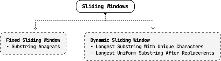
Quyi Satr Anagramlari
Quyi Satr Anagramlari
Kichik harfli ingliz harflaridan iborat ikki satr s va t berilgan, s dagi t ning anagrami bo'lgan quyi satrlar sonini qaytaring.
Anagram — boshqa so'z yoki iboraning barcha asl harflaridan foydalanib ularni qayta tartiblab hosil qilingan so'z yoki ibora.
Misol:
Input: s = 'caabab', t = 'aba'
Output: 2
Tushuntirish: 1-indeksdan boshlanadigan t ning anagrami bor va 2-indeksdan boshlanadigan boshqa anagram bor.
Intuitsiya
Anagram haqidagi fikrlashni berilgan ta'rifni o'zgartirish orqali qayta ifodalashimiz mumkin. s ning quyi satri t ning anagrami sifatida hisoblanadi, agar u t ning barcha belgilarini bir xil chastotada o'z ichiga olsa, lekin har qanday tartibda.
s dagi quyi satrning t ning anagrami bo'lishi uchun u t bilan bir xil uzunlikda bo'lishi kerak (len_t deb belgilaymiz). Bu shuni anglatadiki, biz faqat len_t uzunligidagi quyi satrlarni ko'rib chiqishimiz kerak.
Belgilangan uzunlik len_t dagi barcha quyi satrlarni ko'rib chiqish uchun, belgilangan siljuvchi oyna texnikasidan foydalanishimiz mumkin, chunki oyna len_t dan len_t gacha uzunlikdagi barcha quyi satrlarni ko'radi.

Endi oyna t ning anagrami ekanligini tekshirish usuligina kerak. Anagramda harflar tartibi muhim emasligini esda tuting.
Bu mantiqni misol bilan ko'rib chiqaylik. Siljuvchi oyna algoritmini boshlashdan oldin t ni ifodalash usuli kerak.
expected_freqs — har bir indeksi kichik ingliz harflaridan birini ifodalovchi 26 o'lchamli butun sonlar massivi. Har bir indeksdagi qiymat — t dagi tegishli harfning chastotasi.

Siljuvchi oyna algoritmini o'rnatish uchun quyidagi komponentlarni aniqlaymiz:
- Chap va o'ng ko'rsatkichlar: Oyna chegaralarini aniqlash uchun ikkovini satr boshida ishga tushiring.
- window_freqs: Oyna ichidagi belgilar chastotasini kuzatib borish uchun 26 o'lchamli massiv.
- count: Aniqlangan anagramlar sonini hisoblash uchun o'zgaruvchi saqlang.
Oynani siljitishdan oldin uni len_t ga kengaytirish kerak. Buni o'ng ko'rsatkichni oldinga siljitish orqali amalga oshirish mumkin.



Oyna len_t ga kengayganida, expected_freqs va window_freqs bir xil ekanligini tekshirish orqali t ning anagrami ekanligini tekshirishimiz mumkin.
Ushbu oynani satr bo'ylab siljitish uchun har iteratsiyada chap va o'ng ko'rsatkichlarni bir qadam oldinga siljiting.
![Image represents a Python-like array assignment statement. The statement `expected_freqs = [...]` assigns a numerical array to the variable `expected_freqs`. The array is enclosed in square brackets `[]` and contains numerical values representing frequencies. Specifically, the first element is 2, associated with the character 'a'; the second is 1, associated with 'b'; the third is 0, associated with 'c'; and the remaining elements (indicated by an ellipsis '...') are all 0, extending up to and including the element associated with the character 'z'. The characters 'a' through 'z' are shown below the corresponding frequency values, indicating that the array likely represents the expected frequencies of each letter in the alphabet. There are no URLs or parameters present.](https://bytebytego.com/images/courses/coding-patterns/sliding-windows/substring-anagrams/image-05-01-6-ITVC2B3I.svg?dpl=dpl_Gs7zfM6MUzjTBjcjps1LqXtb9QmD)
![Image represents a data flow diagram illustrating a comparison process. On the left, two labeled boxes, 'left' and 'right,' point downwards with arrows to a light-blue rectangular box containing the character sequence 'c a a b a b'. This sequence appears to be a data window. To the right, the variable `window_freqs` is defined and assigned an array-like value `[2 0 1 ... 0]`, where the subscripts 'a', 'b', 'c', and 'z' indicate that the array represents the frequencies of characters 'a', 'b', 'c', and so on, up to 'z' within the window. The ellipsis (...) denotes that the array continues with frequencies for characters not explicitly shown. Below, a dashed-line box shows a comparison: `window_freqs != expected_freqs`, indicating that the calculated frequencies (`window_freqs`) are being checked against some pre-defined `expected_freqs`. An arrow labeled 'continue' emerges from this box, suggesting that the process continues if the comparison is true (i.e., the frequencies do not match the expected values).](https://bytebytego.com/images/courses/coding-patterns/sliding-windows/substring-anagrams/image-05-01-7-QSRH6VYW.svg?dpl=dpl_Gs7zfM6MUzjTBjcjps1LqXtb9QmD)
![Image represents a sliding window algorithm visualization. Two orange rectangular boxes labeled 'left' and 'right' point downwards with arrows to a light-blue rectangular box containing a sequence of characters 'c a a b a b'. Dashed lines extend from the arrows to indicate the window's boundaries. The 'left' pointer is positioned at the 'a' and the 'right' pointer at the 'b', defining the current window. Above, a list `window_freqs = [2 1 0 ... 0]` shows the frequency count of characters within the window (2 'a's, 1 'b', 0 'c', etc., up to 'z'). To the right, a light-grey box depicts a conditional check: `window_freqs == expected_freqs`, implying a comparison with a pre-defined frequency array (`expected_freqs`). If the condition is true, a counter `count` is incremented (`count += 1`). The diagram illustrates how the window moves across the character sequence, updating `window_freqs` and checking for matches against `expected_freqs` at each step.](https://bytebytego.com/images/courses/coding-patterns/sliding-windows/substring-anagrams/image-05-01-8-SCASOCXD.svg?dpl=dpl_Gs7zfM6MUzjTBjcjps1LqXtb9QmD)
![Image represents a sliding window algorithm segment. Two orange rectangular boxes labeled 'left' and 'right' point downwards with arrows to a light-blue rectangular box containing the character sequence 'a b a'. Dashed arrows indicate the window's movement. The character 'c' precedes the window, and 'b' follows it. To the right, 'window_freqs = [2<sub>a</sub> 1<sub>b</sub> 0<sub>c</sub> ... 0<sub>z</sub>]' shows a frequency array; '2' indicates two occurrences of 'a' within the window, '1' shows one 'b', and '0' represents zero occurrences of 'c' and all other characters (represented by '...'). A light-grey dashed-line box displays the condition 'window_freqs == expected_freqs' which, if true, increments a counter: 'count += 1'. The diagram illustrates how the algorithm checks character frequencies within a sliding window against an expected frequency distribution ('expected_freqs'), updating a counter when a match is found.](https://bytebytego.com/images/courses/coding-patterns/sliding-windows/substring-anagrams/image-05-01-9-ODV3Y2HX.svg?dpl=dpl_Gs7zfM6MUzjTBjcjps1LqXtb9QmD)
![Image represents a sliding window algorithm visualization. Two orange rectangular boxes labeled 'left' and 'right' point downwards via orange arrows to a light-blue rectangular box containing the character sequence 'c a a b'. Dotted orange lines indicate the window's movement. Above, 'window_freqs = [1 2 0 ... 0]' shows an array representing the frequency of characters ('a', 'b', 'c', ..., 'z') within the current window, with 'a' having frequency 1, 'b' having frequency 2, and others having frequency 0. A light-grey dashed-line box displays the condition 'window_freqs != expected_freqs' and an arrow pointing right labeled 'continue,' indicating that if the window's character frequencies do not match the 'expected_freqs' (not shown), the algorithm continues processing. The overall diagram illustrates a step in a character frequency-based algorithm where a sliding window is used to compare observed frequencies against expected frequencies.](https://bytebytego.com/images/courses/coding-patterns/sliding-windows/substring-anagrams/image-05-01-10-DDZFQ4JV.svg?dpl=dpl_Gs7zfM6MUzjTBjcjps1LqXtb9QmD)
len_t uzunligidagi barcha quyi satrlarni qayta ishlashni tugatganimizdan so'ng, anagramlar sonini ifodalovchi count ni qaytarishimiz mumkin.
Kichik bir optimizatsiya — t uzunligi s uzunligidan katta bo'lsa 0 qaytarish, chunki bu holda anagram hosil qilib bo'lmaydi.
Amalga oshirish
Python da kichik harfli ingliz harfining 26 element massivdagi indeksini topish uchun ord(belgi) - ord('a') dan foydalanishimiz mumkin.
def substring_anagrams(s: str, t: str) -> int:
    len_s, len_t = len(s), len(t)
    if len_t > len_s:
        return 0
    count = 0
    expected_freqs, window_freqs = [0] * 26, [0] * 26
    # Populate 'expected_freqs' with the characters in string 't'.
    for c in t:
        expected_freqs[ord(c) - ord('a')] += 1
    left = right = 0
    while right < len_s:
        # Add the character at the right pointer to 'window_freqs' before sliding the
        # window.
        window_freqs[ord(s[right]) - ord('a')] += 1
        # If the window has reached the expected fixed length, we advance the left
        # pointer as well as the right pointer to slide the window.
        if right - left + 1 == len_t:
            if window_freqs == expected_freqs:
                count += 1
            # Remove the character at the left pointer from 'window_freqs' before
            # advancing the left pointer.
            window_freqs[ord(s[left]) - ord('a')] -= 1
            left += 1
        right += 1
    return count
Murakkablik Tahlili
Vaqt murakkabligi: substring_anagrams ning vaqt murakkabligi O(n), bu yerda n s uzunligini bildiradi.
- expected_freqs massivini to'ldirish O(m) vaqt oladi, bu yerda m t uzunligini bildiradi. m n dan kichik kafolatlanganligidan, O(m) = O(n).
- Keyin, s satrini ikkita ko'rsatkich bilan chiziqli ko'rib chiqamiz, bu O(n) vaqt oladi.
- E'tibor bering, har iteratsiyada ikki chastota massivi o'rtasida bajarilgan taqqoslash (expected_freqs va window_freqs) doimiy O(26) = O(1) vaqt oladi.
Xotira murakkabligi: Har bir chastota massivi faqat 26 elementni o'z ichiga olganligi sababli xotira murakkabligi O(1).
Noyob Belgilardan Iborat Eng Uzun Quyi Satr
Noyob Belgilardan Iborat Eng Uzun Quyi Satr
Satr berilgan, faqat noyob belgilardan iborat eng uzun quyi satrining uzunligini aniqlang.
Misol:
Input: s = 'abcba'
Output: 3
Tushuntirish: "abc" quyi satri noyob belgilarni o'z ichiga olgan 3 uzunlikdagi eng uzun quyi satrdir ("cba" ham to'g'ri).
Intuitsiya
Qo'pol kuch yondashuvi barcha mumkin bo'lgan quyi satrlarni ko'rib chiqib faqat noyob belgilardan iboratini tekshirishni o'z ichiga oladi.
- Quyi satrning noyobligini tekshirish, quyi satrni ko'rib chiqib hash to'plamdan foydalanib O(n) vaqtda amalga oshirilishi mumkin.
- Barcha mumkin bo'lgan quyi satrlar bo'ylab takrorlash O(n²) vaqt oladi.
Bu shuni anglatadiki, qo'pol kuch yondashuvi umuman O(n³) vaqt oladi. Bu juda sekin, asosan quyi satrlar bo'ylab ikki marta takrorlash sababli.
Siljuvchi oyna Siljuvchi oyna yondashuvlari quyi satrlarni o'z ichiga oluvchi masalalar uchun juda foydali. Xususan, dinamik siljuvchi oyna ko'pincha eng uzun yoki eng qisqa quyi satrni topish uchun ishlatiladi.
Ixtiyoriy oynani ikki yo'l bilan tasniflashimiz mumkin. Oyna:
- Faqat noyob belgilardan iborat (takroriy belgilarsiz oyna).
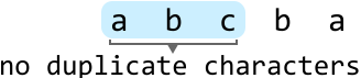
- Kamida bitta belgisi chastotasi 1 dan katta.
Agar A to'g'ri bo'lsa, noyob belgilardan iborat uzunroq oyna topish uchun o'ng ko'rsatkichni oldinga siljitib oynani kengaytirishimiz kerak.
Agar B to'g'ri bo'lsa, oynada takroriy belgi uchragan bo'lsa, oyna takroriy belgini o'z ichiga olmaguncha chap ko'rsatkichni oldinga siljitib oynani toraytirishimiz kerak.
Keling, quyidagi misol bo'yicha bu strategiyani sinab ko'raylik. Oyna ichidagi belgilarni kuzatish uchun hash to'plamni ishga tushiramiz.
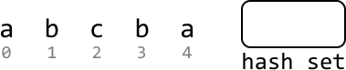
Siljuvchi oyna texnikasini amalga oshirish uchun quyidagilarni o'rnatishimiz kerak:
- Chap va o'ng ko'rsatkichlar: Oyna chegaralarini aniqlash uchun ikkovini satr boshida ishga tushiring.
- hash_set: Oyna ichidagi noyob belgilarni qayd etib borish uchun hash to'plam saqlang, oyna kengaygan yoki toraygan sari uni yangilang.
Endi eng uzun oynani qidirishni boshlaylik. O'ng ko'rsatkichni oldinga siljitib satrning boshidan oynani kengaytiring.




3-indeksdagi 'b' oynada takroriy belgi ekanligini ko'ramiz, chunki 'b' allaqachon hash to'plamda bor.
Takroriy belgi topilgandan so'ng, oyna endi takroriy belgini o'z ichiga olmaguncha chap ko'rsatkichni oldinga siljitib oynani toraytirishimiz kerak.



Oynani yanada kengaytirish o'ng ko'rsatkichni satr chegarasidan tashqariga chiqaradi, bu nuqtada qidirishni to'xtatib eng uzun oynani qaytarishimiz mumkin.
Amalga oshirish
def longest_substring_with_unique_chars(s: str) -> int:
    max_len = 0
    hash_set = set()
    left = right = 0
    while right < len(s):
        # If we encounter a duplicate character in the window, shrink the window until
        # it’s no longer a duplicate.
        while s[right] in hash_set:
            hash_set.remove(s[left])
            left += 1
        # Once there are no more duplicates in the window, update 'max_len' if the
        # current window is larger.
        max_len = max(max_len, right - left + 1)
        hash_set.add(s[right])
        # Expand the window.
        right += 1
    return max_len
Murakkablik Tahlili
Vaqt murakkabligi: longest_substring_with_unique_chars ning vaqt murakkabligi O(n), chunki biz satr bo'ylab chap va o'ng ko'rsatkichlar yordamida o'tamiz.
Xotira murakkabligi: Noyob belgilarni saqlash uchun hash to'plamdan foydalansak, xotira murakkabligi O(m) bo'ladi, bu yerda m o'ziga xos belgilar sonini bildiradi.
Optimizatsiya
Yuqoridagi yondashuv masalani hal qiladi, lekin uni yanada optimallashtirish mumkin. Optimizatsiya — oynani qanday toraytirish bilan bog'liq.
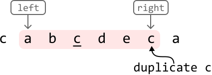
Oldingi yondashuvda takroriy belgi uchragan holatlarda chap ko'rsatkichni takroriy belgini o'z ichiga olmaguncha uzluksiz oldinga siljitib javob beramiz.
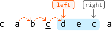
Muhim tushuncha shundan iboratki, biz chap ko'rsatkichni avvalgi 'c' uchrashuvi o'tib ketguncha oldinga siljitdik.
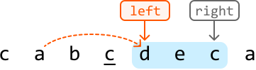
Bu chap ko'rsatkichni oldinga siljitish uchun yangi strategiya beradi: agar o'ng ko'rsatkich oldingi indeksi oynada bo'lgan belgiga duch kelsa, chap ko'rsatkichni to'g'ridan-to'g'ri oldingi indeksdan keyinga ko'chirishimiz mumkin.
Satrning har bir belgisining oldingi indeksini saqlash uchun hash xaritadan (prev_indexes) foydalanishimiz mumkin.
Endi belgining oldingi indeksi oynada ekanligini ta'minlashimiz kerak. Buni uning indeksini chap ko'rsatkich bilan taqqoslash orqali amalga oshiramiz.
- Agar bu indeks chap ko'rsatkichdan keyin bo'lsa, u oyna ichida.
- Agar u chap ko'rsatkichdan oldin bo'lsa, u oynadan tashqarida.
Quyida belgining oyna ichida ekanligini qanday tekshirish ko'rsatilgan:
![Image represents a comparison of how a sliding window algorithm handles duplicate elements within and outside its current view. The diagram is split into two sections, each illustrating a scenario. The left section, titled 'Previous index inside the window:', shows a sequence 'cabcdeca' where a sliding window is highlighted, encompassing 'abcde'. Above this sequence, 'left' and 'right' boxes indicate the window's boundaries. Arrows point from these boxes to the 'a' at the left and 'c' at the right edge of the highlighted section. Below, a box displays the code `prev_indexes['c'] = 3 ≥ left`, indicating that the previous index of 'c' (3) is greater than or equal to the left boundary of the window (implied as 0), signifying that 'c' is already present within the window. Two arrows then point to the conclusions: 'inside window' and 'duplicate in the window'. The right section, titled 'Previous index outside the window:', shows a similar setup with the sequence 'cabcdeca', but the highlighted window is 'abc'. Again, 'left' and 'right' boxes point to the 'd' and 'a' respectively. The code `prev_indexes['a'] = 1 < left` shows that the previous index of 'a' (1) is less than the left boundary, meaning 'a' is outside the current window. Consequently, two arrows point to 'outside window' and 'not a duplicate in the window'. Both sections use color-coding: the highlighted window sections are shaded differently (pink/light blue) to distinguish the current window's contents, and the element being checked for duplication ('c' and 'a') is highlighted in a distinct color (peach/orange).](https://bytebytego.com/images/courses/coding-patterns/sliding-windows/longest-substring-with-unique-characters/image-05-02-14-KQTWCA3E.svg?dpl=dpl_Gs7zfM6MUzjTBjcjps1LqXtb9QmD)
Amalga oshirish - Optimallashtirilgan Yondashuv
def longest_substring_with_unique_chars_optimized(s: str) -> int:
    max_len = 0
    prev_indexes = {}
    left = right = 0
    while right < len(s):
        # If a previous index of the current character is present in the current
        # window, it's a duplicate character in the window.
        if s[right] in prev_indexes and prev_indexes[s[right]] >= left:
            # Shrink the window to exclude the previous occurrence of this character.
            left = prev_indexes[s[right]] + 1
        # Update 'max_len' if the current window is larger.
        max_len = max(max_len, right - left + 1)
        prev_indexes[s[right]] = right
        # Expand the window.
        right += 1
    return max_len
Murakkablik Tahlili
Vaqt murakkabligi: Optimallashtirilgan amalga oshirishning vaqt murakkabligi O(n), chunki biz satrni bir marta kesib o'tamiz.
Xotira murakkabligi: Noyob belgilarni saqlash uchun hash xaritadan foydalansak, xotira murakkabligi O(m) bo'ladi.
Almashtirishlardan Keyin Eng Uzun Bir Xil Quyi Satr
Almashtirishlardan Keyin Eng Uzun Bir Xil Quyi Satr
Bir xil quyi satr — barcha belgilari bir xil bo'lgan satr. Satr va k integer berilgan, satrning ixtiyoriy belgini ko'pi bilan k marta almashtirganingizda erishish mumkin bo'lgan eng uzun bir xil quyi satr uzunligini aniqlang.
Misol:

Input: s = 'aabcdcca', k = 2
Output: 5
Tushuntirish: agar faqat 2 belgini almashtira olsak, erishish mumkin bo'lgan eng uzun bir xil quyi satr — 2-indeksdan boshlanadigan 'ccccc'.
Intuitsiya
Quyi satrning bir xilligini aniqlash Eng uzun bir xil quyi satrni topishga harakat qilishdan oldin, avval quyi satrni bir xil qilish mumkin yoki yo'qligini qanday aniqlashni ko'rib chiqaylik.

Satrni bir xil qilish uchun minimal almashtirish sonini ta'minlash uchun qaysi belgilarni almashtirish kerak?

Asosiy kuzatuv shundan iboratki, bir xillikka erishish uchun zarur bo'lgan minimal almashtirish soni — eng yuqori chastotali belgidan tashqari barcha belgilarni almashtirish orqali olinadi.
Bu shuni ko'rsatadiki, agar quyi satrdagi belgining eng yuqori chastotasini bilsak, almashtirish soni qiymatimizni belgilashimiz mumkin.
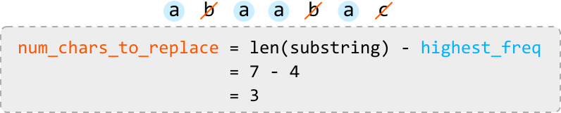
Berilgan quyi satr uchun num_chars_to_replace ni hisoblaganimizdan so'ng, quyi satrni bir xil qilish mumkinligini baholashimiz mumkin:
- Agar num_chars_to_replace ≤ k bo'lsa, quyi satrni bir xil qilish mumkin.
- Agar num_chars_to_replace > k bo'lsa, quyi satrni bir xil qilib bo'lmaydi.
num_chars_to_replace ni hisoblash uchun highest_freq qiymatini bilishimiz kerak. Bu oyna ichidagi belgilar chastotasini kuzatishni talab qiladi.
![Image represents a data flow diagram illustrating the process of finding the highest frequency of a character in a sequence. The input, shown as 'a b c' with a downward arrow indicating data flow, represents a sequence of characters. This input feeds into a table labeled 'freqs', which is a two-column table with headers 'char' and 'freq'. The table shows the character 'a' and its frequency '1'. This table acts as an intermediate data structure storing character frequencies. A separate box contains a code snippet: `highest_freq = max(highest_freq, freqs['a'])`, which calculates the highest frequency encountered so far. The variable `highest_freq` is updated using the `max` function, comparing its current value with the frequency of character 'a' (obtained from the `freqs` table using the key 'a'). The result of this calculation, '1', is displayed below the equation, indicating that the highest frequency found so far is 1. The overall diagram shows how the input sequence is processed to determine the highest character frequency.](https://bytebytego.com/images/courses/coding-patterns/sliding-windows/longest-uniform-substring-after-replacements/image-05-03-4-THMG57YT.svg?dpl=dpl_Gs7zfM6MUzjTBjcjps1LqXtb9QmD)
![Image represents a data flow diagram illustrating a frequency counting algorithm. The input consists of a sequence of characters 'a', 'b', 'b', 'c', depicted by a downward-pointing arrow above the sequence. This input feeds into a table labeled 'freqs,' which is a two-column table with headers 'char' and 'freq.' The table stores the frequency of each character; 'a' has a frequency of 1, and 'b' has a frequency of 1. A separate, light-grey, dashed-bordered box contains a Python code snippet: `highest_freq = max(highest_freq, freqs['b'])`, which calculates the highest frequency encountered so far. The result of this calculation, `= 1`, is shown below the code snippet. The code implies an iterative process where `highest_freq` is updated by comparing it with the frequency of each character in the `freqs` table. The 'b' is used as an example in the code snippet, suggesting the algorithm iterates through each character in the input sequence.](https://bytebytego.com/images/courses/coding-patterns/sliding-windows/longest-uniform-substring-after-replacements/image-05-03-5-2S3UUUAZ.svg?dpl=dpl_Gs7zfM6MUzjTBjcjps1LqXtb9QmD)
![Image represents a data flow diagram illustrating the process of finding the highest frequency of characters in a sequence. The input is a sequence of characters 'a b b c', depicted as a horizontal list. A downward arrow indicates this sequence is processed to generate a frequency table labeled 'freqs'. This table is a 2-column structure with the left column labeled 'char' representing characters and the right column labeled 'freq' representing their frequencies. The table shows 'a' with frequency 1 and 'b' with frequency 2. To the right, a separate box shows a Python-like code snippet calculating the highest frequency. The code `highest_freq = max(highest_freq, freqs['b'])` calculates the maximum frequency by comparing a current `highest_freq` (implicitly initialized to 0 or a lower value not shown) with the frequency of character 'b' (which is 2 from the table). The result, `= 2`, is displayed below, indicating that 2 is the highest frequency found in the input sequence.](https://bytebytego.com/images/courses/coding-patterns/sliding-windows/longest-uniform-substring-after-replacements/image-05-03-6-A7DH6WHO.svg?dpl=dpl_Gs7zfM6MUzjTBjcjps1LqXtb9QmD)
![Image represents a data flow diagram illustrating the process of finding the highest frequency of characters in a sequence. The input is a sequence of characters 'a b b c' shown with a downward arrow indicating data flow into a frequency table labeled 'freqs'. This table is a two-column structure with 'char' representing the character and 'freq' representing its frequency. The table shows 'a' with frequency 1, 'b' with frequency 2, and 'c' with frequency 1. To the right, a calculation is shown: `highest_freq = max(highest_freq, freqs['c']) = 2`. This equation indicates that the `highest_freq` variable is updated by taking the maximum value between its current value (implicitly assumed to be initialized to a value less than or equal to 2) and the frequency of character 'c' (which is 1 from the table), resulting in a final `highest_freq` value of 2. The diagram visually demonstrates how the frequency table is generated from the input sequence and how a maximum frequency is calculated using the table's data.](https://bytebytego.com/images/courses/coding-patterns/sliding-windows/longest-uniform-substring-after-replacements/image-05-03-7-LJGWRHAO.svg?dpl=dpl_Gs7zfM6MUzjTBjcjps1LqXtb9QmD)
Endi quyi satrni bir xil qilish mumkinligini aniqlash vositalariga ega bo'lganligi sababli, keyingi qadam — eng uzun quyi satrni qanday topishni aniqlashdir.
Dinamik siljuvchi oyna Biz siljuvchi oynalar quyi satrlarni o'z ichiga olgan masalalarni hal qilishda foydali bo'lishini bilamiz. Bu masala uchun shart quyidagi:
num_chars_to_replace <= k
Shuning uchun bob kirishida muhokama qilinganidek, dinamik siljuvchi oyna mos bo'lishi mumkin.
Oynani kengaytirish yoki toraytirish usulini aniqlash uchun yuqoridagi shartdan foydalanishimiz mumkin:
- Agar shart bajarilsa (ya'ni oyna haqiqiy), hali ham shartni qondiradigan uzunroq oyna topish uchun oynani kengaytiring.
- Agar shart buzilsa (ya'ni oyna noto'g'ri), shart yana bajarilguncha oynani toraytiring.
Keling, quyidagi misol bo'yicha bu qanday ishlashini ko'rib chiqaylik:

0-indeksda oynaning chap va o'ng chegaralarini belgilashdan boshlang. Oyna haqiqiy bo'lguncha kengaytiring.




Oyna beshinchi belgiga ('d') kengayganida, uni bir xil qilish uchun 3 ta belgini almashtirish kerak bo'ladi.


Oynani toraytirgandan so'ng, highest_freq qiymati hali ham 2, bu endi to'g'ri emas. Esda tuting, highest_freq ni to'g'ri kamaytirish qiyin.
Buning bir echimi — highest_freq ni kamaytirish uchun yangi usul ishlab chiqishdir. Biroq, bu murakkab bo'lishi mumkin.
Bu shuni anglatadiki, noto'g'ri oyna uchra paytda oynani toraytirish o'rniga uni siljitishimiz mumkin, bu samarali ravishda oyna o'lchamini saqlab qoladi.
Bu kuzatuv bilan oldingi mantiqimizni to'g'rilashimiz kerak:
- Agar oyna shartni qondirsa: kengaytiring.
- Agar oyna shartni qondirmasa: siljiting.
Birinchi noto'g'ri oynadagi amalni toraytirish o'rniga siljitish orqali to'g'rilaylik.




Yuqoridagi oyna — yakuniy oyna, chunki uni yanada kengaytirish yoki siljitib bo'lmaydi. Eng uzun haqiqiy oyna 5 uzunlikda.
Amalga oshirish
def longest_uniform_substring_after_replacements(s: str, k: int) -> int:
    freqs = {}
    highest_freq = max_len = 0
    left = right = 0
    while right < len(s):
        # Update the frequency of the character at the right pointer and the highest
        # frequency for the current window.
        freqs[s[right]] = freqs.get(s[right], 0) + 1
        highest_freq = max(highest_freq, freqs[s[right]])
        # Calculate replacements needed for the current window.
        num_chars_to_replace = (right - left + 1) - highest_freq
        # Slide the window if the number of replacements needed exceeds 'k'.
        # The right pointer always gets advanced, so we just need to advance 'left'.
        if num_chars_to_replace > k:
            # Remove the character at the left pointer from the hash map before
            # advancing the left pointer.
            freqs[s[left]] -= 1
            left += 1
        # Since the length of the current window increases or stays the same, assign
        # the length of the current window to 'max_len'.
        max_len = right - left + 1
        # Expand the window.
        right += 1
    return max_len
Murakkablik Tahlili
Vaqt murakkabligi: longest_uniform_substring_after_replacements ning vaqt murakkabligi O(n), bu yerda n satr uzunligini bildiradi.
Xotira murakkabligi: Xotira murakkabligi O(m), bu yerda m satrdagi o'ziga xos belgilar sonini bildiradi.
Ikkilik Qidiruv
Ikkilik Qidiruvga Kirish
Ikkilik Qidiruvga Kirish
Intuitsiya
Aytaylik sizda standart, qog'oz ingliz lug'ati bor va siz 'inheritance' so'zining ta'rifini topmoqchisiz.
Bir yondashuv — sahifani birin-ketin ko'rib chiqish, 'inheritance' bo'lgan sahifaga yetguncha. Lekin bu juda sekin.
Aytaylik siz buni qilib 'M' harfidan boshlanadigan so'zlar sahifasiga tushasiz. 'Inheritance' 'M' dan oldin kelishini tushunib, lug'atning chap yarmiga e'tiboringizni qaratib davom etasiz.

Ikkilik Qidiruvni Amalga oshirish
Ikkilik qidiruv — tartiblangan ma'lumotlar to'plamida qiymatni qidiruvchi algoritm.
Hatto tajribali dasturchilar ham ikkilik qidiruvni to'g'ri amalga oshirishni qiyin deb topishi mumkin, chunki 'shaytonning tafsilotlari' da yashaydi.
- Chap va o'ng chegaraviy o'zgaruvchilar qanday ishga tushirilishi kerak?
- While-tsikldagi chiqish sharti sifatida left < right yoki left ≤ right ishlatish kerakmi?
- Chegaraviy o'zgaruvchilar qanday yangilanishi kerak? left = mid, left = mid + 1, right = mid yoki right = mid - 1 tanlash kerakmi?
Bu bob bu qiyinchiliklarni qanday hal qilishni aniq, intuitiv tarzda ko'rsatadi.
Ixtiyoriy ikkilik qidiruv amalga oshirishini boshlash uchun quyidagilarni bajaring:
- Qidiruv maydonini belgilang.
- Qidiruv maydonini toraytirish uchun tsikl ichidagi xatti-harakatni belgilang.
- While-tsikl uchun chiqish shartini tanlang.
- To'g'ri qiymatni qaytaring.
Keling, bu qadamlarni ko'rib chiqaylik.
1. Qidiruv maydonini belgilash Qidiruv maydoni qidirilayotgan qiymatni o'z ichiga olishi mumkin bo'lgan barcha qiymatlarni o'z ichiga oladi.
![Image represents a visual depiction of a search space within a binary search algorithm. Two orange rectangular boxes labeled 'left' and 'right' are positioned above a horizontal line representing the 'search space'. This space contains a sorted array of integers: [1, 3, 4, 9, 10, 12, 14, 17, 20]. Arrows descend from 'left' and 'right' pointing to the beginning and end of the array, respectively. An orange line underneath the array is labeled 'search space,' indicating the range of values currently being considered during the search. The diagram illustrates the initial state of a binary search, where the algorithm is about to begin its search for a target value within the defined 'search space'.](https://bytebytego.com/images/courses/coding-patterns/binary-search/introduction-to-binary-search/image-06-00-2-PTGT2NKR.svg?dpl=dpl_Gs7zfM6MUzjTBjcjps1LqXtb9QmD)
2. Qidiruv maydonini toraytirish Qidiruv maydonini toraytirish chap yoki o'ng ko'rsatkichni bosqichma-bosqich siljitishni o'z ichiga oladi.
Ikkilik qidiruvning har bir nuqtasida qidiruv maydonimizni qanday toraytirish kerakligini aniqlashimiz kerak. Biz quyidagilardan birini tanlashimiz mumkin:
- Qidiruv maydonini chapga toraytirish (o'ng ko'rsatkichni ichkariga siljitish orqali):

- Qidiruv maydonini o'ngga toraytirish (chap ko'rsatkichni ichkariga siljitish orqali):

O'rta nuqtadan foydalanish Chap yoki o'ng ko'rsatkichni siljitishni o'rta nuqtadagi qiymatga qarab hal qilamiz.

Ikkilik qidiruvning har bir iteratsiyasida berilishi kerak bo'lgan asosiy savol: qidirilayotgan qiymat o'rta nuqtaning chapidami yoki o'ngidami?
Umumiy g'oya shundan iborat: agar qidirayotgan qiymat o'rta nuqtaning o'ngida bo'lsa, qidiruv maydonini o'ngga tomon toraytiring.
Qidiruv maydonini o'ngga toraytirish uchun ikkita variant mavjud:
- left = mid + 1

Buni o'rta nuqta qiymati qidirayotgan qiymat emasligini aniq bilganimizda va uni chiqarib tashlaymizda qilamiz.
- left = mid Buni o'rta nuqta qiymati potentsial ravishda qidirayotgan qiymat bo'lishi mumkin bo'lganda qilamiz.
Chiqarish/qo'shish mantiqi chapga toraytirish uchun ham qo'llaniladi.
O'rta nuqtani hisoblash Ko'p hollarda o'rta nuqta mid = (left + right) // 2 formulasi yordamida hisoblanadi.
3. Chiqish shartini tanlash While-tsikl qachon tugatilishi kerakligini tanlash qiyin bo'lishi mumkin.
- Chiqish sharti left < right bo'lganda, while-tsikl chap va o'ng ko'rsatkichlar uchrashuv qilganda to'xtaydi.
- Boshqa tomondan, left ≤ right chap o'ngdan o'tib ketgandan keyin tugaydi.
![Image represents two diagrams illustrating different loop termination conditions in a search algorithm, likely binary search. The left diagram shows a loop continuing 'while left < right', terminating 'once left == right'. Two orange rectangular boxes labeled 'left' and 'right' are positioned above a series of dots within square brackets [...], representing an array or list. Arrows descend from 'left' and 'right' pointing to separate dots within the array, suggesting the pointers are converging. The right diagram shows a loop continuing 'while left ≤ right', terminating 'once left > right'. Similarly, two orange boxes labeled 'right' and 'left' (note the order change) are above a series of dots within square brackets [...]. Arrows descend from 'right' and 'left', again pointing to separate dots within the array, but this time illustrating the pointers potentially crossing each other before termination. Both diagrams visually represent the iterative process of narrowing down a search space until a condition is met, highlighting the subtle difference in loop conditions and their impact on the final pointer positions.](https://bytebytego.com/images/courses/coding-patterns/binary-search/introduction-to-binary-search/image-06-00-8-KNIVWZTT.svg?dpl=dpl_Gs7zfM6MUzjTBjcjps1LqXtb9QmD)
left < right shartidan chiqqandan keyin chap va o'ng ko'rsatkichlar uchrashuv qilganda, ikkalasi ham bitta qiymatga keladi.
4. To'g'ri qiymatni qaytarish Oldindan ta'kidlab o'tilganidek, while-tsikl qidiruv maydonini bitta qiymatga toraytirganidan keyin tugaydi.

Ushbu yakuniy qiymat — haqiqiy javob mavjud deb faraz qilsak, qidirayotgan javob.
Vaqt Murakkabligi
Ikkilik qidiruvning vaqt murakkabligi O(log(n)), bu yerda n ma'lumotlar to'plamidagi elementlar soni.
Hayotiy Misol
Moliya tizimlarida tranzaksiyalarni qidirish: Moliya tizimlarida ikkilik qidiruvni sanalar bo'yicha tartiblangan yozuvlarda muayyan tranzaksiyani tezda topish uchun ishlatish mumkin.
Bob Mazmuni
Ikkilik qidiruvning ko'plab qo'llanilishlari mavjud va biz turli foydalanishlarni qamrab oluvchi masalalar o'rganamiz.
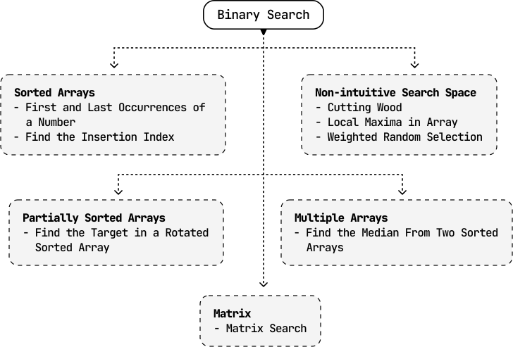
Izohlar
- Kamdan-kam hollarda, masalan yuqori chegarali ikkilik qidiruvda bo'lgani kabi, o'rta nuqtani boshqacha hisoblaymiz.
- Ba'zi noyob vaziyatlarda chap va o'ng ko'rsatkichlar kesishadi, bu ham Birinchi va Oxirgi Uchrashuv masalasida ko'rib chiqiladi.
Kiritish Indeksini Toping
Kiritish Indeksini Toping
Noyob qiymatlarni o'z ichiga olgan tartiblangan massiv va butun son target berilgan.
- Agar massiv target qiymatini o'z ichiga olsa, uning indeksini qaytaring.
- Aks holda, kiritish indeksini qaytaring. Bu target kiritilganda joylashadigan indeks.
Misol 1:
Input: nums = [1, 2, 4, 5, 7, 8, 9], target = 4
Output: 2
Misol 2:
Input: nums = [1, 2, 4, 5, 7, 8, 9], target = 6
Output: 4
Tushuntirish: 6 indeks 4 da joylashishi uchun 5 va 7 orasiga kiritiladi: [1, 2, 4, 5, 6, 7, 8, 9].
Intuitsiya
Bu masalaning maqsadi tartiblangan kiritilgan massiv target qiymatni o'z ichiga oladimi yoki yo'qligiga qarab farqlanadi.
![Image represents two scenarios illustrating a search or insertion operation within a sorted integer array. The left side, titled 'case 1 - target exists in array:', shows an array `[1, 2, 4, 5, 7, 8, 9]` with indices displayed below each element (0-6). The target value, 4, is highlighted in a light green circle at index 2. The right side, titled 'case 2 - target not in array:', displays the array `[1, 2, 4, 5, 7, 8, 9]` with indices (0-6) similarly shown. Here, the target value is 6, which is not present. A light green circle highlights the index 4, indicating where the target value *would* be inserted to maintain the sorted order. A green upward-pointing arrow labeled 'insertion index' points to this highlighted index (4) in the second array. Both cases demonstrate how a target value's presence or absence affects the outcome of a search or insertion algorithm within a sorted array.](https://bytebytego.com/images/courses/coding-patterns/binary-search/find-the-insertion-index/image-06-01-1-7DDXG5I7.svg?dpl=dpl_Gs7zfM6MUzjTBjcjps1LqXtb9QmD)
Target massivda mavjud bo'lmaganda, kiritish indeksi target dan katta yoki teng bo'lgan birinchi qiymatda ekanligini kuzatamiz.
Izlashni boshlashdan oldin target massivda bor yoki yo'qligini bilmasligimizdan, ikkala maqsadni bitta ikkilik qidiruvga birlashtira olamiz.
Massiv tartiblanganligi sababli kerakli indeksni topish uchun ikkilik qidiruvdan foydalanishimiz mumkin.
Ikkilik qidiruv Bu ikkilik qidiruvda biz samarali ravishda shartga mos birinchi qiymatni qidiramiz.
![Image represents a visual explanation of a conditional operation applied to an array. The top displays a conditional statement, `nums[i] >= target ?`, indicating a comparison where each element (`nums[i]`) of an array `nums` is checked against a `target` value. Below are two examples. Each example shows an array of numbers ([1, 2, 4, 5, 7, 8, 9]) and a specified `target` value (4 in the first example and 6 in the second). Underneath each array, a corresponding array of 'F' (False) and 'T' (True) values is shown. These boolean values represent the result of the comparison `nums[i] >= target` for each element. Grey downward-pointing arrows connect each element in the number array to its corresponding boolean value in the result array. In the first example (target = 4), elements less than 4 result in 'F', while elements greater than or equal to 4 result in 'T'. Similarly, in the second example (target = 6), elements less than 6 are 'F', and those greater than or equal to 6 are 'T'. The diagram illustrates how the conditional statement processes each array element to produce a boolean result array.](https://bytebytego.com/images/courses/coding-patterns/binary-search/find-the-insertion-index/image-06-01-2-3CRPXKXO.svg?dpl=dpl_Gs7zfM6MUzjTBjcjps1LqXtb9QmD)
Bu diagrammadan qidirmoqchi bo'lgan qiymat samarali ravishda target ga teng yoki undan katta qiymatlarning quyi chegarasi ekanligini ko'ramiz.
![The image represents two examples illustrating a lower bound in a data structure, likely an array. Each example shows a sequence enclosed in square brackets `[]`. The sequences consist of elements represented by 'F' (in red) and 'T' (in green). In both examples, a single 'T' element, highlighted within a light green circle, is positioned near the beginning of the sequence. An upward-pointing arrow originates from below this circled 'T' and points towards it, labeled 'lower bound'. The first example shows the sequence `[F F F T T T T T]`, while the second example shows `[F F F F F T T T]`. The arrangement demonstrates how the 'T' element acts as a lower bound, indicating a point in the sequence where the condition represented by 'T' begins to hold true. The difference between the two examples highlights that the exact position of the lower bound can vary depending on the data.](https://bytebytego.com/images/courses/coding-patterns/binary-search/find-the-insertion-index/image-06-01-3-FQPOLG6X.svg?dpl=dpl_Gs7zfM6MUzjTBjcjps1LqXtb9QmD)
E'tibor bering, quyi chegarani topish eng chap qiymatni topishga teng. Shu ma'lumot bilan, ikkilik qidiruvni loyihalaylik.
Avval qidiruv maydonini aniqlang. Target massivda mavjud bo'lsa, [0, n-1] oralig'idagi ixtiyoriy indeksda joylashishi mumkin.
Qidiruv maydonini qanday toraytirish kerakligini aniqlash uchun, avval target ni o'z ichiga oluvchi massiv misoliga qarash mumkin.
Target massivda mavjud Quyidagi tartiblangan massivda target qiymat 4 ni qidiring.
![Image represents a visual depiction of a two-pointer approach to searching within a sorted array. Two rectangular boxes labeled 'left' and 'right' are positioned above a sorted integer array [1, 2, 4, 5, 7, 8, 9]. Arrows descend from 'left' and 'right' pointing to the beginning and end of the array respectively. The array elements are numbered below with their indices (0 to 7). To the right of the array, the text 'target = 4' indicates the value being searched for. The diagram illustrates the initial state of a binary search or similar algorithm where the 'left' pointer starts at index 0 and the 'right' pointer starts at index 6, preparing to search for the target value (4) within the array.](https://bytebytego.com/images/courses/coding-patterns/binary-search/find-the-insertion-index/image-06-01-4-7V37KGDJ.svg?dpl=dpl_Gs7zfM6MUzjTBjcjps1LqXtb9QmD)
Dastlab o'rta nuqta 5-elementga joylashgan, bu bizning shartimizni qondiradigan son, ya'ni target dan katta yoki teng.
Shuning uchun, o'rta nuqtani qo'shib, qidiruv maydonini chapga toraytiring (right = mid):
![Image represents a visual depiction of a binary search algorithm step. Three rectangular boxes labeled 'left,' 'mid,' and 'right' are positioned above a numerical array [1, 2, 4, 5, 7, 8, 9], with each box pointing downwards via an arrow to its corresponding index in the array. The 'mid' box is highlighted in light blue, indicating its current focus. The number 4 in the array is highlighted in light green, representing the element at the 'mid' index. A dashed-line rectangle to the right displays a conditional statement: 'nums[mid] ≥ 4 → right = mid,' indicating that if the value at the middle index ('nums[mid]') is greater than or equal to 4, then the 'right' index is updated to the current 'mid' index. This illustrates a step in narrowing down the search space within the array. The numbers below the array represent the indices (0-7) of each element.](https://bytebytego.com/images/courses/coding-patterns/binary-search/find-the-insertion-index/image-06-01-5-ZBUKWPAC.svg?dpl=dpl_Gs7zfM6MUzjTBjcjps1LqXtb9QmD)
![Image represents a visual depiction of a two-pointer approach in array traversal. A rectangular box labeled 'left' points down to a bracketed sequence `[1 2 4 5 7 8 9]`, indicating the starting point of a left pointer. The numbers are indexed below, starting from 0. A second rectangular box labeled 'right' points down to the number 5 within the sequence. A light-green circle highlights the number 4, visually separating the left and right pointers' initial positions. A dashed orange line curves from the number 5 (the right pointer's initial position) to the closing bracket `]`, suggesting the right pointer's traversal direction. The numbers 7, 8, and 9 are shown in lighter gray, indicating they are yet to be processed. The overall arrangement illustrates the initial state of a two-pointer algorithm operating on an array, where the left pointer starts at index 0 and the right pointer starts at index 3, with the right pointer moving towards the end of the array.](https://bytebytego.com/images/courses/coding-patterns/binary-search/find-the-insertion-index/image-06-01-6-5WWETRZI.svg?dpl=dpl_Gs7zfM6MUzjTBjcjps1LqXtb9QmD)
Endi o'rta nuqta 2-elementga joylashgan. Quyi chegara target dan katta yoki teng qiymat bo'lishi kerak.
Shuning uchun, o'rta nuqtani chiqarib, qidiruv maydonini o'ngga toraytiring:
![Image represents a visual depiction of a step within a binary search algorithm. Three rectangular boxes labeled 'left,' 'mid,' and 'right' are positioned above a numerical array [1, 2, 4, 5, 7, 8, 9], with index numbers displayed below each element. Arrows descend from 'left,' 'mid,' and 'right' pointing to the array elements 1, 2, and 5 respectively. The element at index 2 (value 4) is highlighted in light green. To the right, a dashed-line box contains a conditional statement: 'nums[mid] < 4 → left = mid + 1,' indicating that if the value at the middle index (nums[mid], which is 4 in this case) is less than 4, then the 'left' index should be updated to 'mid + 1'. This illustrates how the algorithm adjusts the search space based on the comparison of the middle element with the target value (implicitly 4 in this example).](https://bytebytego.com/images/courses/coding-patterns/binary-search/find-the-insertion-index/image-06-01-7-U2YJETFM.svg?dpl=dpl_Gs7zfM6MUzjTBjcjps1LqXtb9QmD)
![Image represents a visual depiction of a data structure manipulation, possibly illustrating an algorithm or a coding pattern. A horizontal line represents a sequence of numbered elements, bracketed by '[' and ']'. The numbers 1 through 9 are shown along this line, with numbers 0 through 7 displayed below as indices. A light green circle labeled '4' highlights an element within the sequence. Two rectangular boxes, one orange labeled 'left' and one gray labeled 'right', are positioned above the sequence. A solid orange arrow descends from 'left' pointing to the element '4', indicating a potential insertion or modification at that position. A solid gray arrow descends from 'right' pointing to the element '5', suggesting a similar action. A dashed orange curved line connects the 'left' box to the element '4', implying a possible search or selection process leading to the element '4' from the left side. The overall diagram likely illustrates how elements are accessed or manipulated within a sequence based on directional cues ('left' and 'right'), potentially demonstrating concepts like array indexing or list traversal.](https://bytebytego.com/images/courses/coding-patterns/binary-search/find-the-insertion-index/image-06-01-8-UGTV47SZ.svg?dpl=dpl_Gs7zfM6MUzjTBjcjps1LqXtb9QmD)
Endi o'rta nuqta 4-elementga joylashgan, bu target dan katta yoki teng shartini qondiradi.
![Image represents a visual depiction of a step within a binary search algorithm. At the top, three rectangular boxes labeled 'left,' 'mid,' and 'right' are shown horizontally. Light blue arrows descend from 'mid' to highlight its index within a numerical array displayed below. This array, enclosed in square brackets `[ ]`, contains the numbers 1, 2, 4, 5, 7, 8, 9, with their indices (0-7) shown faintly beneath. The number 4, at index 2, is highlighted with a light green circle. The array's element at the index indicated by 'mid' (which is 4) is being compared to the value 4. To the right, a light gray, dashed-bordered rectangle displays the conditional logic: `nums[mid] ≥ 4 → right = mid`, indicating that if the value at the middle index (`nums[mid]`) is greater than or equal to 4, then the 'right' index is updated to be equal to the 'mid' index. This illustrates a step in narrowing down the search space within the binary search.](https://bytebytego.com/images/courses/coding-patterns/binary-search/find-the-insertion-index/image-06-01-9-35EGI4ZZ.svg?dpl=dpl_Gs7zfM6MUzjTBjcjps1LqXtb9QmD)
![Image represents a visual depiction of a data structure, possibly an array or list, with elements numbered 1 through 9, enclosed within square brackets '[' and ']'. A light-green circle labeled '4' highlights the element at index 2. Two rectangular boxes, one labeled 'left' in gray and the other 'right' in orange, indicate directional pointers. A solid gray arrow points from 'left' to the circled '4', while a solid orange arrow points from 'right' to the circled '4'. A dashed orange curved arrow originates near the circled '4' and points back towards it, suggesting an iterative or cyclical process. The numbers below the main line represent the indices of the array elements, ranging from 0 to 7, corresponding to the elements above. The overall diagram illustrates a concept related to accessing or manipulating an element within a data structure, potentially within the context of algorithms like binary search or other pointer-based operations.](https://bytebytego.com/images/courses/coding-patterns/binary-search/find-the-insertion-index/image-06-01-10-EBZUIING.svg?dpl=dpl_Gs7zfM6MUzjTBjcjps1LqXtb9QmD)
Chap va o'ng ko'rsatkichlar uchrashuv qilganida, quyi chegara joylashtirilgan — bu target dan katta yoki teng bo'lgan birinchi qiymat.
Target massivda mavjud emas Yuqoridagi mantiqni target mavjud bo'lmagan quyidagi misol yordamida sinab ko'raylik.
![The image represents a visual depiction of a search for a target value within a numerical array. The top row displays an array of integers enclosed in square brackets: [1, 2, 4, 5, 7, 8, 9]. To the right, separated by a comma, is the text 'target = 6,' indicating that the goal is to find the number 6 within the array. The bottom row shows the indices of the array elements, ranging from 0 to 7, corresponding to each element's position. A light-green circle highlights the index '4' which is below the number '7' in the array, suggesting that the algorithm is currently examining or has examined this element during its search for the target value 6. The absence of the target value (6) in the array is implicitly shown by the highlighting of an index that does not correspond to the target value.](https://bytebytego.com/images/courses/coding-patterns/binary-search/find-the-insertion-index/image-06-01-11-ZSNM22N6.svg?dpl=dpl_Gs7zfM6MUzjTBjcjps1LqXtb9QmD)
![Image represents a visual depiction of a binary search algorithm step. Three rectangular boxes labeled 'left,' 'mid,' and 'right' are positioned above a numerical array [1, 2, 4, 5, 7, 8, 9], with each box pointing downwards via an arrow to its corresponding element's index in the array. The 'mid' box is highlighted in light blue, indicating its current focus. Below the array, indices 0 through 7 are displayed. The element at index 4 (value 7) is highlighted in light green. A dashed-line rectangular box contains the conditional statement 'nums[mid] < 6 → left = mid + 1,' illustrating that if the value at the middle index ('nums[mid]') is less than 6, the 'left' index is updated to 'mid + 1,' effectively narrowing the search space to the right half of the array for the next iteration. The arrows visually represent the data flow and the conditional logic of the algorithm.](https://bytebytego.com/images/courses/coding-patterns/binary-search/find-the-insertion-index/image-06-01-12-ZRXBWE7X.svg?dpl=dpl_Gs7zfM6MUzjTBjcjps1LqXtb9QmD)
![Image represents a visual depiction of a data structure, possibly an array or list, illustrating a coding pattern. A numerical sequence [1, 2, 4, 5, 7, 8, 9] is displayed, with numbers positioned along a horizontal axis labeled with indices 0 through 7 below. An orange dashed line curves from a point between 1 and 2, reaching a point above the number 7. An orange rectangle labeled 'left' is connected by a downward-pointing arrow to the number 7. A gray rectangle labeled 'right' is connected by a downward-pointing arrow to the number 9. A light green circle containing the number 4 is positioned below the number 7, possibly indicating an index or a specific element's value. The dashed line suggests a connection or operation involving the 'left' pointer and the element at index 4, potentially illustrating a search or traversal algorithm within the data structure.](https://bytebytego.com/images/courses/coding-patterns/binary-search/find-the-insertion-index/image-06-01-13-TANKUKKW.svg?dpl=dpl_Gs7zfM6MUzjTBjcjps1LqXtb9QmD)
![Image represents a visual depiction of a step within a binary search algorithm. The top shows three labeled boxes: 'left,' 'mid' (highlighted in cyan), and 'right.' Arrows descend from 'left' and 'mid' pointing to the numbers 7 and 8 respectively, within a numerical array [1, 2, 4, 5, 7, 8, 9]. The array's indices are shown below, with index 4 highlighted in light green, corresponding to the value 7. An arrow descends from 'right' to the number 9 in the array. A separate, light-grey, dashed-bordered box displays the conditional logic: 'nums[mid] ≥ 6 → right = mid,' indicating that if the element at the middle index (`mid`) is greater than or equal to 6, then the 'right' index is updated to the value of `mid`. This illustrates how the algorithm adjusts the search space based on the comparison of the middle element with a target value (implicitly 6 in this case).](https://bytebytego.com/images/courses/coding-patterns/binary-search/find-the-insertion-index/image-06-01-14-VUMKKPLG.svg?dpl=dpl_Gs7zfM6MUzjTBjcjps1LqXtb9QmD)
![Image represents a visual depiction of a coding pattern, likely illustrating array indexing or pointer manipulation. A numbered array, represented by `[1 2 4 5 7 8 9]`, is shown with indices displayed below (0-7). Two rectangular boxes labeled 'left' (gray) and 'right' (orange) point downwards to array elements 7 and 8 respectively. A downward-pointing arrow from 'left' indicates selection of element 7, while a similar arrow from 'right' points to element 8. A dashed orange curved line connects 'right' to the array's closing bracket `]`, suggesting a potential iteration or traversal to the end of the array. A small light green circle containing the number 4 is positioned below the element 7, possibly indicating an additional variable or index value related to the 'left' pointer. The overall arrangement suggests a scenario where two pointers, 'left' and 'right,' operate on the array, potentially for searching, sorting, or other array-processing algorithms.](https://bytebytego.com/images/courses/coding-patterns/binary-search/find-the-insertion-index/image-06-01-15-JZCCGIWY.svg?dpl=dpl_Gs7zfM6MUzjTBjcjps1LqXtb9QmD)
![Image represents a visual depiction of a step within a binary search algorithm. A numerical array `[1, 2, 4, 5, 7, 8, 9]` is shown, with indices displayed below. Three labeled boxes, 'left,' 'mid' (highlighted in cyan), and 'right,' are positioned above the array, indicating pointers or indices. Arrows from 'left,' 'mid,' and 'right' point downwards to the elements 7, 7, and 8 respectively in the array. The element at index 4 (value 7) is highlighted in light green, suggesting it's the current `mid` point. A separate, dashed-bordered box displays a conditional statement: `nums[mid] ≥ 6 → right = mid`, indicating that if the value at the `mid` index (7 in this case) is greater than or equal to 6, then the `right` pointer is updated to the `mid` index's value. This illustrates a decision-making step within the algorithm's iterative process of narrowing down the search space.](https://bytebytego.com/images/courses/coding-patterns/binary-search/find-the-insertion-index/image-06-01-16-ANHMI7MN.svg?dpl=dpl_Gs7zfM6MUzjTBjcjps1LqXtb9QmD)
![Image represents a visual depiction of a binary search algorithm operating on a sorted array. A numbered array [1, 2, 4, 5, 7, 8, 9] is shown, with numbers 0 through 7 displayed below as indices. A light green circle labeled '4' indicates the midpoint of the array after an initial search. Two rectangular boxes, one labeled 'left' in gray and the other 'right' in orange, point downwards with arrows to the number '7' within the array. The 'left' arrow indicates a search starting from the left side of the array, while the 'right' arrow indicates a search from the right. A dashed orange arrow from 'right' to '7' shows the right pointer converging on '7'. This illustrates how the algorithm iteratively narrows down the search space by comparing the target value (implicitly understood to be 7) with the middle element, adjusting the search boundaries ('left' and 'right' pointers) until the target is found.](https://bytebytego.com/images/courses/coding-patterns/binary-search/find-the-insertion-index/image-06-01-17-TLBBPQAB.svg?dpl=dpl_Gs7zfM6MUzjTBjcjps1LqXtb9QmD)
Ko'rib turganingizdek, ikkilik qidiruv oxiriga yetgach, qidiruv maydonini bitta qiymatga toraytirdik.
Xulosa Aniqlik uchun, qidiruv maydonini torayltirishda uchraydigan ikki asosiy ssenariyni xulosalaymiz.
1-holat: O'rta nuqta qiymati target dan katta yoki unga teng, bu quyi chegara o'rta nuqtada yoki undan chapda ekanligini bildiradi.
![Image represents a visual depiction of a binary search algorithm's step. At the top, a code snippet shows the conditional statement `if nums[mid] ≥ target: right = mid;`, indicating that if the element at the middle index (`mid`) of the array `nums` is greater than or equal to the target value, the `right` boundary of the search space is updated to `mid`. Below, two arrays, `[1, 2, 4, 5, 7, 8, 9]` and `[1, 2, 4, 5, 7, 8, 9]`, represent the initial and updated search spaces respectively. Index numbers are shown below each element. Boxes labeled 'left,' 'mid,' and 'right' indicate the boundaries of the search space. Arrows show the flow of information: 'left' points to the first element (index 0), 'mid' points to the element at index 3 (value 5), and 'right' initially points to the last element (index 7). In the updated array, a dashed orange line connects the previous `right` pointer (index 7) to the new `right` pointer (index 3), visually representing the narrowing of the search space due to the condition being met. The element at `mid` (value 5) is highlighted, and the number 4 is highlighted in both arrays to emphasize its position relative to the `mid` and `left` pointers.](https://bytebytego.com/images/courses/coding-patterns/binary-search/find-the-insertion-index/image-06-01-18-2JR5FV4I.svg?dpl=dpl_Gs7zfM6MUzjTBjcjps1LqXtb9QmD)
2-holat: O'rta nuqta qiymati target dan kichik, bu quyi chegara o'rta nuqtaning o'ngida ekanligini bildiradi.
![Image represents a visual depiction of a binary search algorithm's iteration. The top shows a code snippet: `if nums[mid] < target: left = mid + 1`, indicating a conditional statement within the algorithm where if the value at the middle index (`mid`) of the array `nums` is less than the target value, the `left` boundary is updated to `mid + 1`. Below, two arrays `[1, 2, 4, 5, 7, 8, 9]` are shown, representing the search space. The first array shows the initial state with index numbers (0-7) beneath each element. Arrows labeled 'left,' 'mid,' and 'right' point to the respective boundaries of the search space (1, 5, and 9 initially). The second array illustrates the next iteration. The `mid` pointer has moved, and the `left` pointer has shifted to the right (indicated by an orange dashed arrow) because the condition `nums[mid] < target` was true. The `right` pointer remains unchanged. The index numbers are again shown below the array. The number 8 is highlighted in light green in both arrays, suggesting it might be the target value or relevant to the search.](https://bytebytego.com/images/courses/coding-patterns/binary-search/find-the-insertion-index/image-06-01-19-CKCIRTJR.svg?dpl=dpl_Gs7zfM6MUzjTBjcjps1LqXtb9QmD)
Amalga oshirish
from typing import List

def find_the_insertion_index(nums: List[int], target: int) -> int:
    left, right = 0, len(nums)
    while left < right:
        mid = (left + right) // 2
        # If the midpoint value is greater than or equal to the target, the lower
        # bound is either at the midpoint, or to its left.
        if nums[mid] >= target:
            right = mid
        # The midpoint value is less than the target, indicating the lower bound is
        # somewhere to the right.
        else:
            left = mid + 1
    return left
Murakkablik Tahlili
Vaqt murakkabligi: find_the_insertion_index ning vaqt murakkabligi O(log(n)), chunki qidiruv maydoni har iteratsiyada yarmiga qisqaradi.
Xotira murakkabligi: Xotira murakkabligi O(1).
Sonning Birinchi va Oxirgi Uchrashuvi
Sonning Birinchi va Oxirgi Uchrashuvi
O'smaydigan tartibda tartiblangan butun sonlar massivi berilgan, target qiymatining birinchi va oxirgi indekslarini qaytaring.
Misol 1:
Input: nums = [1, 2, 3, 4, 4, 4, 5, 6, 7, 8, 9, 10, 11],
       target = 4
Output: [3, 5]
Tushuntirish: 4 sonining birinchi va oxirgi uchrashuvi mos ravishda 3 va 5 indekslarda.
Intuitsiya
Bu masalaga qo'pol kuch yechimi birinchi va oxirgi uchrashuvni topish uchun chiziqli qidiruvni o'z ichiga oladi.
Bu yerda ikkilik qidiruvdan foydalanishning qiyinligi — bir xil qiymatning ikkita alohida uchrashuvini topish zarurligida.
Yechim topishga yordam berish uchun masala samarali ravishda bizdan targetning quyi va yuqori chegarasini topishni so'rashi muhim.
![Image represents a sequence of integers from 1 to 11, displayed in two rows. The top row shows the integers [1, 2, 3, 4, 4, 4, 5, 6, 7, 8, 9, 10, 11], with the three consecutive '4's highlighted in a light peach/orange rectangle. The bottom row displays the corresponding indices, ranging from 0 to 12. Two orange downward-pointing arrows connect the bottom row to labels below. The arrow originating from index 3 points to the label 'lower bound,' and the arrow originating from index 5 points to the label 'upper bound,' indicating that the highlighted sequence of three '4's starts at the lower bound (index 3) and ends at the upper bound (index 5).](https://bytebytego.com/images/courses/coding-patterns/binary-search/first-and-last-occurrences-of-a-number/image-06-02-1-BFVXIASI.svg?dpl=dpl_Gs7zfM6MUzjTBjcjps1LqXtb9QmD)
Bu masalani ikki asosiy qadamda hal qilish mumkinligini ko'rsatadi:
- Target ning quyi chegarasini topish uchun ikkilik qidiruv bajaring.
- Target ning yuqori chegarasini topish uchun ikkilik qidiruv bajaring.
Quyi chegara ikkilik qidiruv Target ning boshlanish pozitsiyasini topish uchun avval qidiruv maydonini aniqlaymiz.
Keyingi, qidiruv maydonini qanday toraytirish kerakligini aniqlaylik. Ikkilik qidiruvning har bir nuqtasida o'rta nuqta qiymatining uchta holati mavjud:
- target dan katta bo'lganida
- target dan kichik bo'lganida
- target ga teng bo'lganida
Har bir holatda, target ning o'rta nuqtaga nisbatan qayerda joylashganligini o'ylab ko'ring.
O'rta nuqta qiymati target dan katta O'rta nuqta qiymati katta bo'lsa, target o'rta nuqtaning chapida ekanligini bildiradi.
Buni qilganda o'rta nuqtani qidiruv maydonidan chiqarish mumkin (right = mid - 1), chunki u quyi chegara bo'lolmaydi.
![Image represents a visual depiction of a step within a binary search algorithm or a similar search/sorting process operating on a numerical array. The array `nums` is displayed horizontally, with elements [1, 2, 3, 4, 4, 4, 5, 6, 7, 8, 9, 10, 11]. Index values are shown below each element (0-12). Three labeled pointers, 'left', 'mid', and 'right', indicate array boundaries or positions. 'left' points to the beginning of the array (index 0), 'right' points to the end (index 12), and 'mid' points to element 4 at index 3 (highlighted in light green). A dashed box below the array displays a conditional statement: `nums[mid] > 4`. An arrow indicates that if this condition is true, then the 'right' pointer is updated to `right = mid - 1`, effectively narrowing the search space to the left half of the array. The visual arrangement clearly shows the pointers' positions and how the condition affects the 'right' pointer's movement, illustrating a key step in a divide-and-conquer approach to searching or sorting.](https://bytebytego.com/images/courses/coding-patterns/binary-search/first-and-last-occurrences-of-a-number/image-06-02-2-R4PR2PPX.svg?dpl=dpl_Gs7zfM6MUzjTBjcjps1LqXtb9QmD)

O'rta nuqta qiymati target dan kichik O'rta nuqta qiymati kichikroq bo'lsa, target o'rta nuqtaning o'ngida ekanligini bildiradi.
![Image represents a visual depiction of a binary search algorithm's step. Three labeled boxes, 'left,' 'mid,' and 'right,' point downwards to respective indices within a numbered array [1, 2, 3, 4, 4, 4, 5, 6, 7, 8, 9, 10, 11]. The array's indices are shown below the numbers, ranging from 0 to 12. 'left' points to index 0 (value 1), 'mid' points to index 2 (value 3), highlighted in light green, and 'right' points to index 5 (value 4). A dashed box at the bottom displays the condition `nums[mid] < 4`, which evaluates to true because 3 < 4. An arrow indicates this condition leads to the assignment `left = mid + 1`, updating the 'left' index to 3 (the next index after 'mid'). The visual emphasizes the iterative process of narrowing down the search space within the array based on the comparison of the middle element with the target value (implicitly 4).](https://bytebytego.com/images/courses/coding-patterns/binary-search/first-and-last-occurrences-of-a-number/image-06-02-4-5S36355O.svg?dpl=dpl_Gs7zfM6MUzjTBjcjps1LqXtb9QmD)

O'rta nuqta qiymati target ga teng Endi qiziqarli narsa boshlanadi. O'rta nuqta qiymati target ga teng bo'lganda ikkita imkoniyat mavjud:
- Bu target qiymatining quyi chegarasi.
- Bu quyi chegara emas, shuning uchun quyi chegara chapda biroz narida.
Hozircha qaysi imkoniyat to'g'ri ekanligini bilmaymiz, shuning uchun o'rta nuqtani qo'shib qidiruv maydonini chapga toraytirish kerak.
![Image represents a visual depiction of a binary search algorithm step. At the top, three rectangular boxes labeled 'left,' 'mid' (highlighted in light blue), and 'right' indicate index pointers. Arrows descend from each box, pointing to a numbered sequence [1, 2, 3, 4, 4, 4, 5, 6, 7, 8, 9, 10, 11] displayed below. The numbers are positioned above their corresponding indices (0-12) shown in a lighter gray. The 'mid' pointer points to the value '4' at index 4. A light green circle highlights the '4' at index 3, visually representing the 'left' pointer's position. The 'right' pointer also points to a '4' at index 5. At the bottom, a dashed-line box displays the code snippet 'nums[mid] == 4 → right = mid,' illustrating the algorithm's logic: if the value at the middle index ('nums[mid]') equals the target value (4), then the 'right' pointer is updated to the 'mid' index. This signifies that the search space has been narrowed down.](https://bytebytego.com/images/courses/coding-patterns/binary-search/first-and-last-occurrences-of-a-number/image-06-02-6-M7LHMWPK.svg?dpl=dpl_Gs7zfM6MUzjTBjcjps1LqXtb9QmD)

Keyingi o'rta nuqta uchun ham target ga teng bo'lganida bu fikrni davom ettiring:
![Image represents a visual depiction of a binary search algorithm step. A numbered array [1, 2, 3, 4, 4, 4, 5, 6, 7, 8, 9, 10, 11] is shown with indices displayed below. Three labeled boxes, 'left,' 'mid,' and 'right,' represent pointers to array elements. A light-green circle highlights the element at index 3, which is the value 4, indicating the current 'mid' point. Arrows point from 'left' and 'right' to the 'mid' element, showing how these pointers converge. Below the array, a code snippet 'nums[mid] == 4 → right = mid' illustrates the algorithm's logic: if the value at the midpoint ('nums[mid]') equals the target value (4), the 'right' pointer is updated to the current 'mid' index, effectively narrowing the search space to the left half of the array for the next iteration.](https://bytebytego.com/images/courses/coding-patterns/binary-search/first-and-last-occurrences-of-a-number/image-06-02-8-YF3MIF75.svg?dpl=dpl_Gs7zfM6MUzjTBjcjps1LqXtb9QmD)

Chap va o'ng ko'rsatkichlar uchrashuv qilgandan keyin yakuniy qiymat target ning quyi chegarasi.
Yuqori chegara ikkilik qidiruv Bu va quyi chegara ikkilik qidiruvi orasida ko'p o'xshashlik bor.
Mantiqidagi farq o'rta nuqta target ga teng bo'lganda paydo bo'ladi, chunki endi yuqori chegarani qidiryapmiz.
O'rta nuqta qiymati target ga teng Quyi chegara ikkilik qidiruviga o'xshab, ikkita imkoniyat mavjud:
![Image represents a visual depiction of a binary search algorithm step. At the top, three rectangular boxes labeled 'left,' 'mid' (highlighted in light blue), and 'right' are shown. Arrows descend from each box, pointing to elements within a numbered array represented horizontally below. The array, indexed from 0 to 12, contains the numbers [1, 2, 3, 4, 4, 4, 5, 6, 7, 8, 9, 10, 11]. The 'left' arrow points to the number 4 at index 3, the 'mid' arrow points to the number 4 at index 4, and the 'right' arrow points to the number 4 at index 5 (highlighted in light green). At the bottom, a gray dashed box displays the code snippet 'nums[mid] == 4 -> left = mid,' indicating that because the value at the middle index ('mid') is equal to 4, the 'left' index is updated to equal the 'mid' index. This illustrates a step in the binary search where the target value (4) has been found at the middle index, resulting in an update of the search space.](https://bytebytego.com/images/courses/coding-patterns/binary-search/first-and-last-occurrences-of-a-number/image-06-02-10-ITFBJLGX.svg?dpl=dpl_Gs7zfM6MUzjTBjcjps1LqXtb9QmD)

Keyingi o'rta nuqta qiymatlari uchun bu mantiqni davom ettirsak, g'alati narsa yuz berishini sezamiz:
![Image represents a visual depiction of a binary search algorithm step. A numbered array [1, 2, 3, 4, 4, 5, 6, 7, 8, 9, 10, 11] is shown, with indices displayed below. Above the array, three rectangular boxes labeled 'left,' 'mid,' and 'right' represent pointers or indices within the array. A light-green circle highlights the element at index 4 (value 4). Arrows point from 'left' and 'right' to this highlighted element, indicating the current midpoint of the search. Below the array, a code snippet 'nums[mid] == 4 → left = mid' shows that the value at the midpoint (nums[mid]) is 4, and consequently, the 'left' pointer is updated to equal the 'mid' pointer. This suggests the algorithm is searching for a value (likely 4), and this step shows the narrowing of the search space by updating the 'left' pointer.](https://bytebytego.com/images/courses/coding-patterns/binary-search/first-and-last-occurrences-of-a-number/image-06-02-12-FSTGFCOE.svg?dpl=dpl_Gs7zfM6MUzjTBjcjps1LqXtb9QmD)

![Image represents a visual depiction of a binary search algorithm step. At the top, three rectangular boxes labeled 'left,' 'mid,' and 'right' represent index pointers within a sorted numerical array shown below. The array, depicted as a number line from 0 to 12, contains the numbers 1 through 11. A light green circle highlights the element at index 4, which holds the value 4. Light blue arrows point from 'mid' to this highlighted element, indicating that the midpoint of the search is currently at index 4. Below the array, a dashed box displays the code snippet 'nums[mid] == 4 -> left = mid,' illustrating that because the value at the midpoint (nums[mid]) equals the target value (4), the 'left' pointer is updated to equal the 'mid' pointer. This signifies that the search has successfully found the target value at the midpoint.](https://bytebytego.com/images/courses/coding-patterns/binary-search/first-and-last-occurrences-of-a-number/image-06-02-14-L6TIEPOU.svg?dpl=dpl_Gs7zfM6MUzjTBjcjps1LqXtb9QmD)
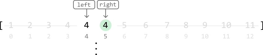
Biz cheksiz siklga tushib qolgan ko'rinamiz, chap ko'rsatkich pozitsiyasi doim midga teng bo'lib qoladi.
Cheksiz siklni tuzatish Chap va o'ng ko'rsatkichlar to'g'ridan-to'g'ri yonma-yon bo'lganda, mid chap ko'rsatkichga yo'naltiriladi.

Bir operatsiyamiz left = mid bo'lganligi sababli, chap va mid doim tengligicha qoladigan cheksiz siklga tushib qolamiz.
O'rta nuqta o'ngga o'zgarganda, yuqori chegara ikkilik qidiruvida cheksiz sikldan qochamiz.
- mid endi chap ko'rsatkich emas, o'ng ko'rsatkich pozitsiyasida joylashganligi sababli chap ko'rsatkich haqida tashvishlanishimiz shart emas.
- O'ng ko'rsatkich mid ga o'rnatilmaganligi sababli o'ng ko'rsatkich bilan cheksiz siklga duch kelmaymiz.
O'rta nuqtaning o'ngga yo'naltirishi mid = (left + right) // 2 + 1 formulasi yordamida erishilishi mumkin:

Endi, left = mid bajarilishi qidiruv maydonini to'g'ri toraytirish imkonini beradi.
Umumiy qoida sifatida, yuqori chegara ikkilik qidiruvida mid ni o'ngga yo'naltirish kerak.
Keling, bir xil misolga ushbu o'zgarishni qo'llab, nima bo'lishini ko'raylik:
![Image represents a visual depiction of a step within a binary search algorithm. At the top, three rectangular boxes labeled 'left,' 'mid' (highlighted in light blue), and 'right' are shown. Arrows descend from each box, pointing to elements within a numbered array visualized horizontally below. The array contains the numbers 1 through 11, with indices displayed below. The 'left' arrow points to the number 4 at index 3, the 'mid' arrow points to the number 4 at index 4, and the 'right' arrow points to the number 4 at index 5 (highlighted in light green). At the bottom, a dashed-line box displays the code snippet 'nums[mid] == 4 → left = mid,' indicating that because the value at the middle index ('mid') of the array is equal to 4, the 'left' index is updated to be equal to the 'mid' index. This illustrates a key step in the binary search where the search space is narrowed based on the comparison of the middle element with the target value.](https://bytebytego.com/images/courses/coding-patterns/binary-search/first-and-last-occurrences-of-a-number/image-06-02-18-D76CB5JI.svg?dpl=dpl_Gs7zfM6MUzjTBjcjps1LqXtb9QmD)
![Image represents a visual depiction of a step within a binary search algorithm. A numbered array, indexed from 0 to 12, is shown with values implicitly represented by their index positions. The array segment from index 0 to 12 is displayed. Three labeled boxes, 'left' (orange), 'mid' (cyan), and 'right' (gray), represent index pointers. Arrows indicate that 'left' and 'right' initially point to indices 3 and 5 respectively, while 'mid' points to index 4. A light green circle highlights the element at index 4, which has a value of 4. A dashed orange arrow shows a tentative movement of the 'left' pointer. A solid cyan arrow shows the movement of the 'mid' pointer. A separate box displays the condition `nums[mid] == 4 -> left = mid`, indicating that because the element at the midpoint (index 4) equals 4, the 'left' pointer is updated to the value of the 'mid' pointer (index 4). This illustrates a step where the target value is found at the midpoint, resulting in the update of the 'left' pointer.](https://bytebytego.com/images/courses/coding-patterns/binary-search/first-and-last-occurrences-of-a-number/image-06-02-19-VPJANQOD.svg?dpl=dpl_Gs7zfM6MUzjTBjcjps1LqXtb9QmD)

Ko'rib turganingizdek, cheksiz sikldan qochdik, chap va o'ng ko'rsatkichlar yuqori chegara indeksida uchrashuv qildi.
Agar target mavjud bo'lmasa Ikkala algoritmning ham oxirgi qadami — joylashtirilgan yakuniy qiymatlar haqiqatan ham target qiymatlari ekanligini tekshirishdir.
Amalga oshirish
from typing import List

def first_and_last_occurrences_of_a_number(nums: List[int], target: int) -> List[int]:
    lower_bound = lower_bound_binary_search(nums, target)
    upper_bound = upper_bound_binary_search(nums, target)
    return [lower_bound, upper_bound]

def lower_bound_binary_search(nums: List[int], target: int) -> int:
    left, right = 0, len(nums) - 1
    while left < right:
        mid = (left + right) // 2
        if nums[mid] > target:
            right = mid - 1
        elif nums[mid] < target:
            left = mid + 1
        else:
            right = mid
    return left if nums and nums[left] == target else -1

def upper_bound_binary_search(nums: List[int], target: int) -> int:
    left, right = 0, len(nums) - 1
    while left < right:
        # In upper-bound binary search, bias the midpoint to the right.
        mid = (left + right) // 2 + 1
        if nums[mid] > target:
            right = mid - 1
        elif nums[mid] < target:
            left = mid + 1
        else:
            left = mid
    # If the target doesn’t exist in the array, then it's possible that
    # 'left = mid + 1' places the left pointer outside the array when `mid == n - 1`.
    # So, we use the right pointer in the return statement instead.
    return right if nums and nums[right] == target else -1
Murakkablik Tahlili
Vaqt murakkabligi: lower_bound_binary_search va upper_bound_binary_search ning vaqt murakkabligi O(log(n)).
Xotira murakkabligi: Xotira murakkabligi O(1).
Intervyu Maslahat
Maslahat: Algoritmingizni har doim sinab ko'ring. Ikkilik qidiruvni amalga oshirish qiyin bo'lishi mumkin. Eng yaxshi usul — chekkadagi holatlar bilan sinab ko'rish.
Yog'och Kesish
Yog'och Kesish
Daraxtlarning balandliklarini ifodalovchi massiv va kesish uchun kerakli yog'och uzunligini ifodalovchi k butun son berilgan.
Ushbu vazifa uchun yog'och kesish mashinasi ma'lum H balandligiga o'rnatiladi. Mashina har bir daraxtning H dan yuqori qismini kesadi.
Yog'ochchi massivdagi eng baland daraxt balandligidan yuqori o'rnatila olmasligini taxmin qiling.
Misol:
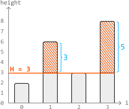
Input: heights = [2, 6, 3, 8], k = 7
Output: 3
Tushuntirish: Kamida k = 7 metr yog'och beruvchi eng yuqori mumkin H balandligi 3, bu 5 metr yog'och beradi.
Cheklovlar:
- Kamida k metr yog'och olish har doim mumkin.
- Kamida bitta daraxt bor.
Intuitsiya
Dastlab bu masalaning nima uchun Ikkilik Qidiruv bobida ekanligini g'alati deb topishingiz mumkin. Berilgan kiritilgan ma'lumotlar... daraxtlar massivi.
Keling [2, 6, 3, 8] balandlikli to'rtta daraxtni vizuallashtiraylik va k = 7 deb faraz qilaylik:
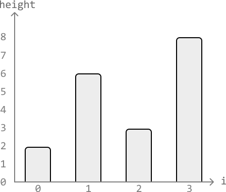
Yuqoridagi eng baland daraxt balandligi 8. Shuning uchun H balandligi o'rnatish 0 dan 8 gacha ixtiyoriy balandlikka o'rnatilishi mumkin:
- Eng ko'p yog'och H = 0 da kesiladi, barcha daraxtlar pastdan kesilganda.
- Eng kam yog'och H = 8 da kesiladi, hech qanday yog'och kesilmaydi.
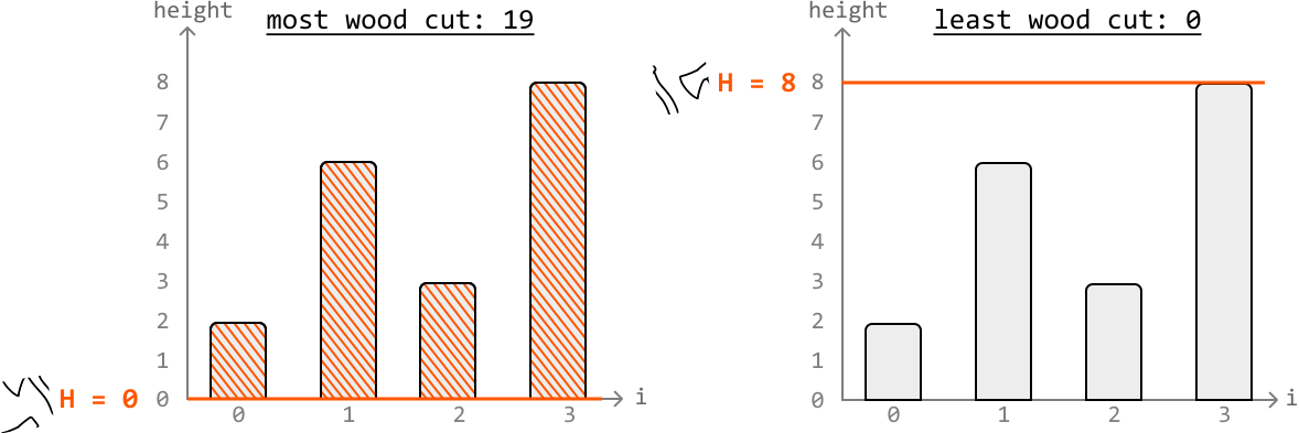
Yog'ochchi H balandligini 0 dan 8 gacha asta-sekin oshirish kamroq va kamroq yog'och beradi.
Balandlik o'rnatish yetarli yog'och berishini aniqlash Berilgan H balandlik o'rnatishi yetarli yog'och berishini aniqlaydigan funksiya kerak.
Bu funksiyani cuts_enough_wood(H, k) deb ataymiz, u har bir daraxtni H balandligida kesib olingan umumiy yog'ochni hisoblab chiqadi.
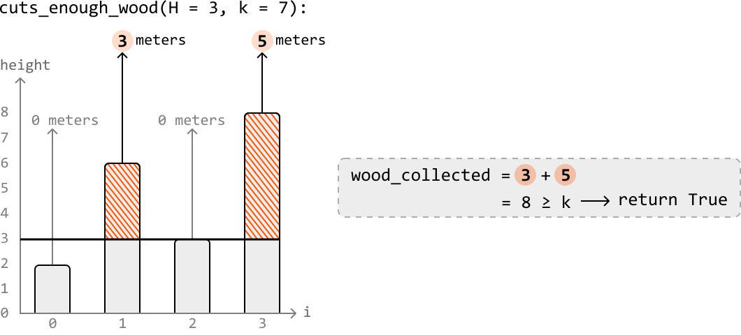
Bu funksiyani 0 dan 8 gacha H ning barcha qiymatlari uchun qo'llash quyidagi natijani beradi, bu yerda haqiqiy qiymatlar kamida k metr yog'ochni kesish mumkin bo'lgan balandliklarni bildiradi.

H ning 0 dan 8 gacha har bir qiymati uchun cuts_enough_wood ni chaqirish mumkin, to kamida k metr yog'ochni kesuvchi eng yuqori qiymatga yetguncha.
Bu tartiblangan ketma-ketlik bo'lgani uchun ikkilik qidiruvdan foydalanishimiz kerak.
Ikkilik qidiruv Maqsad kamida k metr yog'och kesuvchi H ning oxirgi qiymatini topishdir. Boshqacha aytganda, bu yuqori chegarali ikkilik qidiruv muammosidir.

Shuning uchun yuqori chegara ikkilik qidiruvidan foydalanishimiz kerak.
Avval qidiruv maydonini aniqlaymiz. Qidiruv maydonimiz 0 dan massivdagi maksimal qiymatgacha H ning barcha qiymatlarini qamrab olishi kerak.
Qidiruv maydonini qanday toraytirish kerakligini aniqlash uchun, chap va o'ng ko'rsatkichlarni massiv chegaralariga qo'yib quyidagi misoldan foydalanamiz.

Dastlab o'rta nuqta H = 4 ga o'rnatilgan. cuts_enough_wood(4, k) ni chaqirganda u false qaytaradi. Bu yuqori chegara to'liq H = 4 ning chapida ekanligini bildiradi.
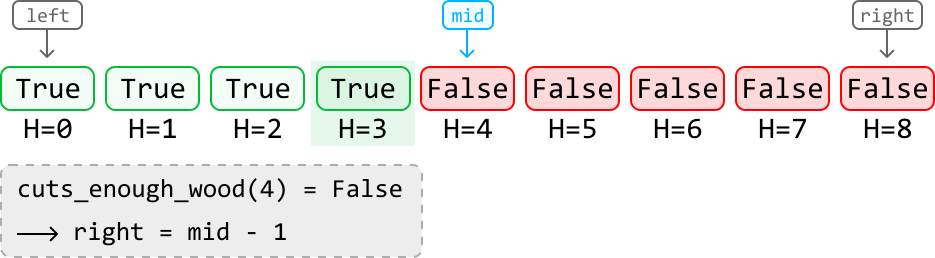

Keyingi o'rta nuqta H = 2 ga o'rnatilgan. cuts_enough_wood(2, k) ni chaqirganda u true qaytaradi. Bu yuqori chegara H = 2 da yoki undan o'ngda ekanligini bildiradi.
Shuning uchun, o'rta nuqtani qo'shib, qidiruv maydonini o'ngga toraytiring:
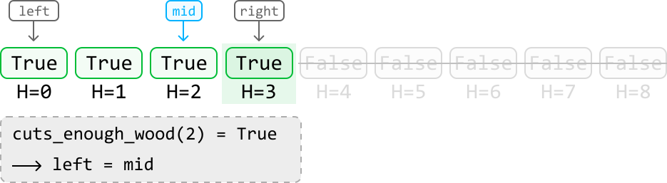

Keyingi o'rta nuqta H = 3 ga o'rnatilgan. cuts_enough_wood(3, k) ni chaqirganda true qaytaradi. Shuning uchun, qidiruv maydonini o'ngga toraytiring.
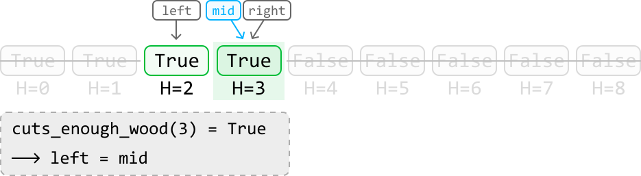

Chap va o'ng ko'rsatkichlar uchrashuv qilganda, kamida k metr yog'och kesuvchi yuqori chegara balandlik o'rnatish joylashtirildi.
Xulosa 1-holat: O'rta nuqta kamida k metr yog'och kesish imkonini beruvchi balandlikda o'rnatilgan, bu yuqori chegara H = O'rta nuqta da yoki o'ngida ekanligini bildiradi.
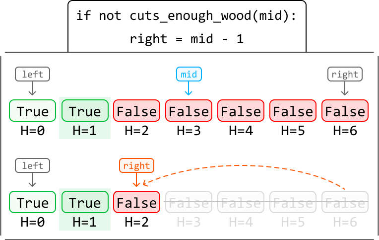
2-holat: O'rta nuqta yetarli yog'och kesish imkonini bermaydigan balandlikda, bu yuqori chegara o'rta nuqtaning chapida ekanligini bildiradi.
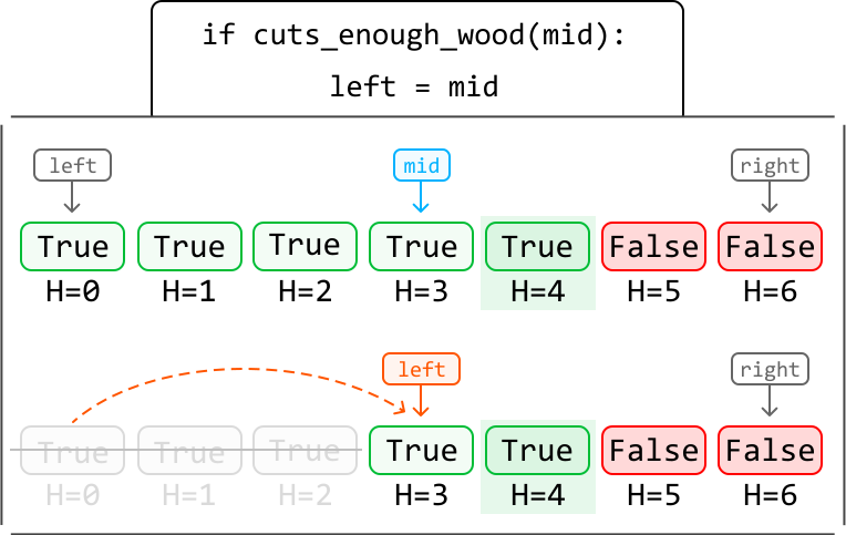
Amalga oshirish
from typing import List

def cutting_wood(heights: List[int], k: int) -> int:
    left, right = 0, max(heights)
    while left < right:
        # Bias the midpoint to the right during the upper-bound binary search.
        mid = (left + right) // 2 + 1
        if cuts_enough_wood(mid, k, heights):
            left = mid
        else:
            right = mid - 1
    return right

# Determine if the current value of 'H' cuts at least 'k' meters of wood.
def cuts_enough_wood(H: int, k: int, heights: List[int]) -> bool:
    wood_collected = 0
    for height in heights:
        if height > H:
            wood_collected += (height - H)
    return wood_collected >= k
Murakkablik Tahlili
Vaqt murakkabligi: cutting_wood ning vaqt murakkabligi O(n log(m)), bu yerda m massivdagi maksimal daraxt balandligi.
Xotira murakkabligi: Xotira murakkabligi O(1).
Aylantirilgan Tartiblangan Massivda Maqsadni Toping
Aylantirilgan Tartiblangan Massivda Maqsadni Toping
Aylantirilgan tartiblangan massiv — o'sish tartibida tartiblangan sonlar massivi bo'lib, uning bir qismi oxiridan boshiga ko'chirilgan.
Noyob sonlardan iborat aylantirilgan tartiblangan massiv berilgan, target qiymatning indeksini qaytaring. Agar target mavjud bo'lmasa, -1 qaytaring.
Misol:
Input: nums = [8, 9, 1, 2, 3, 4, 5, 6, 7], target = 1
Output: 2
Intuitsiya
Sodda yechim — target topilguncha kiritilgan massivni ko'rib chiqishdir. Bu O(n) vaqt oladi.
Avval ikkilik qidiruv uchun qidiruv maydonini aniqlang. Target massivning ixtiyoriy joyida bo'lishi mumkin, shuning uchun qidiruv maydoni [0, n-1] bo'ladi.
Endi qidiruv maydonini qanday toraytirish kerakligini aniqlaylik — massiv aylantirilganligini hisobga olsak, bu qiziqarli muammo.
![Image represents a depiction of a search problem. The top row shows a list of integers, represented as an array `[8, 9, 1, 2, 3, 4, 5, 6, 7]`, enclosed in square brackets. This array is implicitly indexed, with the indices 0 through 8 shown in a smaller font below the corresponding array elements. The text 'target = 1' indicates that the goal is to find the element with the value 1 within the array. The arrangement visually suggests a linear search scenario, where the algorithm would sequentially check each element of the array until it finds the element matching the target value. There are no explicit connections or information flow depicted beyond the visual representation of the array and the target value.](https://bytebytego.com/images/courses/coding-patterns/binary-search/find-the-target-in-a-rotated-sorted-array/image-06-04-1-THCGS3H2.svg?dpl=dpl_Gs7zfM6MUzjTBjcjps1LqXtb9QmD)
Chap va o'ng ko'rsatkichlarni massiv chegaralariga qo'yib, birinchi o'rta nuqta qiymatini ko'rib chiqing.
![Image represents a visual depiction of array partitioning, likely within the context of a divide-and-conquer algorithm. Three rectangular boxes labeled 'left' (orange), 'mid' (light blue), and 'right' (orange) are positioned above a numerical array [8, 9, 1, 2, 3, 4, 5, 6, 7]. Arrows descend from each box, pointing to the array elements. The 'left' box's arrow points to the first two elements (8 and 9), the 'mid' box's arrow points to the element 3 (the middle element in this example), and the 'right' box's arrow points to the last two elements (6 and 7). The numbers beneath the array (0-8) represent the indices of the array elements. The diagram illustrates how an array is conceptually divided into sections, possibly for recursive processing, with the 'mid' pointer potentially indicating a pivot point or a division boundary.](https://bytebytego.com/images/courses/coding-patterns/binary-search/find-the-target-in-a-rotated-sorted-array/image-06-04-2-WZYLMWDI.svg?dpl=dpl_Gs7zfM6MUzjTBjcjps1LqXtb9QmD)
Oddiy tartiblangan massivda qidiruv maydonini chapga yoki o'ngga toraytirish kerakligini mantiqiy baholashimiz mumkin edi.
Qidiruv maydonini o'rta nuqtaning chapiga yoki o'ngiga toraytirish kerakligini aniqlash uchun ikki quyi massivdan biri tartiblangan bo'lishidan foydalanamiz.
![Image represents a visual depiction of a sorting algorithm, likely merge sort, illustrating the merging of two sorted subarrays. The top section shows an unsorted array [8, 9, 1, 2, 3, 4, 5, 6, 7] divided into three parts: 'left' [8, 9, 1, 2], 'mid' [3], and 'right' [4, 5, 6, 7]. Arrows labeled 'left', 'mid', and 'right' point downwards to their respective subarrays, indicating the input to the merging process. The bottom section displays a bar chart representing the same numbers. The 'left' subarray's bars are taller and unsorted, while the 'right' subarray's bars are shorter, light blue, and sorted in ascending order, as indicated by the label 'ascending' below the chart. The bars visually represent the magnitude of each number. The merging process is implied by the juxtaposition of the sorted 'right' subarray with the unsorted 'left' subarray, suggesting the next step would be to combine them into a single sorted array.](https://bytebytego.com/images/courses/coding-patterns/binary-search/find-the-target-in-a-rotated-sorted-array/image-06-04-3-VJSSAMAW.svg?dpl=dpl_Gs7zfM6MUzjTBjcjps1LqXtb9QmD)
Bu yerda [mid : right] quyi massivi o'sish tartibida tartiblangan ekanligini ko'ramiz. Tartiblanganligi sababli, unda target ning qayerda joylashganini mantiqiy baholashimiz mumkin.
Shuning uchun, o'rta nuqtani chiqarib qidiruv maydonini chapga toraytiring (right = mid - 1):
![Image represents a visual depiction of a two-pointer approach in a coding pattern, likely for array traversal or manipulation. A gray rectangular box labeled 'left' points down to a numerical array [8, 9, 1, 2, 3, 4, 5, 6, 7]. Below the array, gray numbers 0 through 8 indicate the indices. An orange rectangular box labeled 'right' points down to the element '2' in the array, signifying its initial position. A dashed orange line curves from the element '2' to the element '7', illustrating a connection or interaction between these two points. The numbers 3, 4, 5, 6, and 7 are shown in gray, indicating they are part of the array but not directly involved in the initial pointer positions. The overall diagram suggests a process where two pointers, one starting at the left and one at a position within the array, interact or move through the array, possibly to find a specific element or perform a comparison.](https://bytebytego.com/images/courses/coding-patterns/binary-search/find-the-target-in-a-rotated-sorted-array/image-06-04-4-AER2PN6L.svg?dpl=dpl_Gs7zfM6MUzjTBjcjps1LqXtb9QmD)
O'rta nuqta qiymatini chiqarib tashlaganimizning sababi — u target ga teng emas edi va shuning uchun javob bo'lmasligi kerak edi.
Misol bilan davom etaylik.
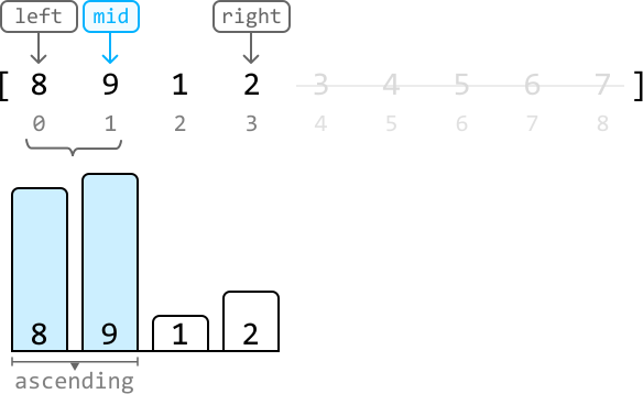
Bu safar tartiblangan quyi massiv chap quyi massiv, [left : mid]. Shuning uchun, bu quyi massivdan target ning qayerda joylashganini aniqlash uchun foydalanishimiz mumkin.
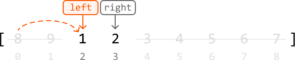
Yana, o'rta nuqta qiymatini (9) target ga teng emasligi sababli chiqarib tashladik.
Nihoyat, o'rta nuqtada target topildi, shuning uchun uning indeksini (mid) qaytaramiz:
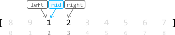
Xulosa Muhokamada muhim strategiya ko'rinadi: ikki quyi massiv orasida, [left : mid] va [mid : right], ulardan biri doim tartiblangan bo'ladi.
Quyi massivlarni tekshirishdan oldin avval target ni o'rta nuqtadagi qiymat bilan solishtiring. Agar ular teng bo'lsa, mid ni qaytaring.
1-holat: chap quyi massiv, [left : mid], tartiblangan
- Agar target ushbu chap quyi massiv oralig'ida bo'lsa, qidiruv maydonini chapga toraytiring.
- Aks holda, qidiruv maydonini o'ngga toraytiring.
![Image represents a visual explanation of a binary search algorithm's behavior, specifically Case 1 where the subarray [left:mid) is sorted. The top section shows an initial array [3, 4, 5, 6, 7, 1, 2] represented as bars with their values labeled. Gray boxes labeled 'left' and 'right' indicate the initial search boundaries. A light-blue box labeled 'mid' highlights the middle element (6). A downward-pointing arrow from 'left' points to 3, and another from 'right' points to 2. A cyan arrow points from 'mid' to the element 6. The bottom-left shows pseudocode: `if nums[left] <= target < nums[mid] → right = mid - 1` else `→ left = mid + 1`. This logic dictates how the search boundaries ('left' and 'right') are adjusted based on the target value's relationship to the middle element. The bottom-right shows two subsequent steps of the algorithm. The first shows the array after the first iteration, with the 'right' pointer moved to the element 5. The second shows the array after the second iteration, with the 'left' pointer moved to the element 7. Gray curved arrows connect the pseudocode to these steps, illustrating how the algorithm updates the search space based on the condition. The dashed orange lines show the movement of the 'right' and 'left' pointers across the array during the iterations.](https://bytebytego.com/images/courses/coding-patterns/binary-search/find-the-target-in-a-rotated-sorted-array/image-06-04-8-FNBAW2B4.svg?dpl=dpl_Gs7zfM6MUzjTBjcjps1LqXtb9QmD)
2-holat: o'ng quyi massiv, [mid : right] tartiblangan
- Agar target ushbu o'ng quyi massiv oralig'ida bo'lsa, qidiruv maydonini o'ngga toraytiring.
- Aks holda, qidiruv maydonini chapga toraytiring.
![Image represents a visual explanation of a coding pattern, specifically a case within a binary search algorithm. The top section shows an array of numbers [6, 7, 1, 2, 3, 4, 5] partitioned into three sections labeled 'left,' 'mid,' and 'right.' The 'mid' section (containing 2) is highlighted in light blue. Arrows indicate the boundaries of these sections. Below this, two further examples illustrate the algorithm's iterative steps. The first shows the 'left' pointer moving to the right, encompassing the 'mid' section, after a comparison. The second example shows the 'right' pointer moving to the left, after a different comparison. A gray box at the bottom contains pseudocode: `if nums[mid] < target < nums[right] → left = mid + 1` and `else → right = mid - 1`. This code describes the conditional logic determining the pointer movement based on the target value's relationship to the values at the 'mid' and 'right' indices. Curved arrows in orange and gray connect the array representations to show the pointer movements ('left' in orange, 'right' in gray) during the algorithm's iterations. The overall diagram demonstrates how the algorithm iteratively narrows the search space by adjusting the 'left' and 'right' pointers until the target is found or the search space is exhausted.](https://bytebytego.com/images/courses/coding-patterns/binary-search/find-the-target-in-a-rotated-sorted-array/image-06-04-9-IOH6QXUD.svg?dpl=dpl_Gs7zfM6MUzjTBjcjps1LqXtb9QmD)
Ikkala quyi massiv ham tartiblangan holatga duch kelish mumkin. Bu holda farq qilmaydi.
Nihoyat, massiv target qiymatni o'z ichiga olmasligi mumkinligini ham hisobga olish kerak. Bu holda while-tsikl tugatilgandan keyin -1 qaytaramiz.
Amalga oshirish
from typing import List

def find_the_target_in_a_rotated_sorted_array(nums: List[int], target: int) -> int:
    left, right = 0, len(nums) - 1
    while left < right:
        mid = (left + right) // 2
        if nums[mid] == target:
            return mid
        # If the left subarray [left : mid] is sorted, check if the target falls in
        # this range. If it does, search the left subarray. Otherwise, search the
        # right.
        elif nums[left] <= nums[mid]:
            if nums[left] <= target < nums[mid]:
                right = mid - 1
            else:
                left = mid + 1
        # If the right subarray [mid : right] is sorted, check if the target falls
        # in this range. If it does, search the right subarray. Otherwise, search the
        # left.
        else:
            if nums[mid] < target <= nums[right]:
                left = mid + 1
            else:
                right = mid - 1
    # If the target is found in the array, return it’s index. Otherwise, return -1.
    return left if nums and nums[left] == target else -1
Murakkablik Tahlili
Vaqt murakkabligi: find_the_target_in_a_rotated_sorted_array ning vaqt murakkabligi O(log(n)).
Xotira murakkabligi: Xotira murakkabligi O(1).
Ikki Tartiblangan Massivdan O'rta Qiymatni Toping
Ikki Tartiblangan Massivdan O'rta Qiymatni Toping
Ikki tartiblangan butun sonlar massivi berilgan, ularning birlashtirilgan tartiblangan massiv kabi o'rta qiymatini toping.
-misol:
Input: nums1 = [0, 2, 5, 6, 8], nums2 = [1, 3, 7]
Output: 4.0
Tushuntirish: Ikkala massivni birlashtirish [0, 1, 2, 3, 5, 6, 7, 8] natijasini beradi, bu juft uzunlikka ega. O'rta qiymat = (3 + 5) / 2 = 4.0.
-misol:
Input: nums1 = [0, 2, 5, 6, 8], nums2 = [1, 3, 7, 9]
Output: 5.0
Tushuntirish: Ikkala massivni birlashtirish [0, 1, 2, 3, 5, 6, 7, 8, 9] natijasini beradi, bu toq uzunlikka ega. O'rta qiymat = 5.
Cheklovlar:
- Kirish massivlaridan kamida bittasida element bo'ladi.
Fikrlash tarzi
Bu masalaning qo'pol kuch yondashuvi ikkala massivni birlashtirish va o'rta qiymatni topishni o'z ichiga oladi. Ammo bu O(n+m) vaqt murakkabligiga olib keladi.
Ushbu tushuntirishda "umumiy uzunlik" ikkala massivning birlashtirilgan uzunligini bildiradi.
Juft umumiy uzunlikka ega quyidagi ikki massivni ko'rib chiqing:
![Image represents two Python list assignments. The first line assigns a list named `nums1` containing the integer elements 0, 2, 5, 6, and 8. The second line assigns a list named `nums2` containing the integer elements 1, 3, and 7. Both lists are presented using standard Python list notation, with square brackets `[]` enclosing the elements, and commas separating them. There is no explicit connection or data flow shown between the two lists; they are simply defined independently of each other.](https://bytebytego.com/images/courses/coding-patterns/binary-search/find-the-median-from-two-sorted-arrays/image-06-05-1-WP4AB67J.svg?dpl=dpl_Gs7zfM6MUzjTBjcjps1LqXtb9QmD)
Bu ikkala massiv birlashtirilganda qanday ko'rinishini ko'rsatadi. Keling, ularni chap va o'ng qismlarga bo'lishga harakat qilaylik.
![Image represents a one-dimensional array labeled 'merged array:'. The array is enclosed in square brackets `[]` and contains the following integer elements, listed sequentially: 0, 1, 2, 3, 5, 6, 7, 8. There are no other visible components, connections, or information flows depicted in the image beyond the array itself and its descriptive label. The elements are presented without any apparent structure or organization beyond their numerical order within the array.](https://bytebytego.com/images/courses/coding-patterns/binary-search/find-the-median-from-two-sorted-arrays/image-06-05-2-MGZLD4UC.svg?dpl=dpl_Gs7zfM6MUzjTBjcjps1LqXtb9QmD)
Birlashtirilgan massiv ikkita yarmga bo'linishi mumkinligi kuzatiladi, bu o'rta qiymatni aniqlashga yordam beradi.
![Image represents a visual depiction of splitting an array into two halves. A numerical array, represented by elements [0, 1, 2, 3, 5, 6, 7, 8] enclosed in square brackets, is shown. A dashed-line box visually separates the array into a 'left half' (elements 0, 1, 2, 3) and a 'right half' (elements 5, 6, 7, 8). The element '4' is seemingly absent. The text 'left half' in cyan is positioned below the left half of the array, while 'right half' in orange is below the right half. Upward-pointing arrows connect the end of the left half (element 3) with the text 'end of left half' in cyan above it, and the start of the right half (element 5) with the text 'start of right half' in orange above it. This illustrates the division point and the labeling of the two resulting sub-arrays.](https://bytebytego.com/images/courses/coding-patterns/binary-search/find-the-median-from-two-sorted-arrays/image-06-05-3-DLIVKAMO.svg?dpl=dpl_Gs7zfM6MUzjTBjcjps1LqXtb9QmD)
Bu yerda asosiy muammo — har bir kirish massividagi qaysi qiymatlar chap yoki o'ng yarmga tegishli ekanligini aniqlash.
Ikkala massivni kesish Qaysi qiymatlar qaysi yarmga tegishli ekanligini aniqlash uchun ikkala massivni ham kesib ko'rishimiz mumkin.
![Image represents a visual depiction of a partitioning algorithm, likely quicksort, showing the process of dividing an array into smaller sub-arrays. Three stages are shown, each displaying an array represented as two horizontal rows of numbers enclosed in square brackets `[]`. The top row contains elements `[0, 2, 5, 6, 8]` in all three stages, while the bottom row contains `[1, 3, 7]` which remains constant. The arrays are partitioned using two colored lines: light blue for the 'left partition' and light orange for the 'right partition'. Triangles (pointing upwards) indicate pivot points within each partition. Numbers above the lines indicate the lengths of the partitions. A curved arrow labeled 'slice' shows the movement of the partition boundaries, illustrating how the algorithm iteratively divides the array. The legend clarifies that the arrow indicates data movement from the right partition to the left partition. The initial array is implicitly divided into two partitions based on the pivot. Subsequent stages show the refinement of these partitions, with the final stage suggesting a nearly sorted array.](https://bytebytego.com/images/courses/coding-patterns/binary-search/find-the-median-from-two-sorted-arrays/image-06-05-4-4BIATGYJ.svg?dpl=dpl_Gs7zfM6MUzjTBjcjps1LqXtb9QmD)
Ko'rib turganimizdek, ikkita bo'linmani hosil qilishning bir necha yo'li mavjud.
![Image represents a visual depiction of array splitting or partitioning. The top section shows two 2D arrays, one light blue containing the elements [0, 2] in the first row and [1, 3] in the second, and the other peach-colored containing [5, 6, 8] in the first row and [7] in the second. A vertical line separates these arrays. Light blue horizontal lines with small triangles at their ends indicate the lengths of the rows in the light blue array (2 elements in the top row and 2 in the bottom). Similarly, orange lines with triangles show the lengths of the rows in the peach array (3 elements in the top row and 1 in the bottom). The numbers '2' and '3' above the arrays indicate the lengths of the respective rows. The bottom section displays the same elements arranged as two 1D arrays: a light blue array [0, 1, 2, 3] and a peach array [5, 6, 7, 8], separated by a vertical line, representing the concatenated elements from the original 2D arrays. The diagram illustrates how a larger array might be conceptually divided into smaller sub-arrays, potentially for parallel processing or other algorithmic purposes.](https://bytebytego.com/images/courses/coding-patterns/binary-search/find-the-median-from-two-sorted-arrays/image-06-05-5-CEVQSUY2.svg?dpl=dpl_Gs7zfM6MUzjTBjcjps1LqXtb9QmD)
Buni "to'g'ri kesim" deb ataymiz. To'g'ri kesimni qanday topishni tushuntiramiz.
To'g'ri kesimni aniqlash
Muhim kuzatuv: chap bo'linmadagi barcha qiymatlar o'ng bo'linmadagi barcha qiymatlardan kichik yoki teng bo'lishi kerak.
Buni ikki qismning oxirgi qiymatlarini boshlanish qiymatlari bilan taqqoslash orqali baholashimiz mumkin.
![Image represents a diagram illustrating a coding pattern, likely related to array or list comparisons. The diagram shows two rectangular regions, one light blue and one peach, representing potentially two different arrays or lists. Each region contains several black dots representing elements, and two circled elements labeled L1, L2 (light blue) and R1, R2 (peach). L1 and L2 are positioned at the right edge of their respective regions, while R1 and R2 are positioned at the left edge of their respective regions. A horizontal line connects the right edge of the light blue region to the left edge of the peach region. The text below the diagram specifies a condition to be checked: `(L1 ≤ R1, L1 ≤ R2)` and `(L2 ≤ R1, L2 ≤ R2)`. This indicates a comparison where the values of L1 and L2 (from the light blue region) are checked to see if they are less than or equal to the values of R1 and R2 (from the peach region). The brackets `[` and `]` around the elements suggest that the regions represent ordered sequences, possibly arrays or lists.](https://bytebytego.com/images/courses/coding-patterns/binary-search/find-the-median-from-two-sorted-arrays/image-06-05-6-SQUKHFCH.svg?dpl=dpl_Gs7zfM6MUzjTBjcjps1LqXtb9QmD)
Har bir massivdagi qiymatlar tartiblanganligi sababli, L1 ≤ R1 va L2 ≤ R2 shartlari doimo bajarilishini bilamiz.
![Image represents three examples illustrating a coding pattern, possibly related to array partitioning or range checks. Each example shows a numerical array enclosed in square brackets, partitioned into sub-arrays. The first array in each example is split into two sub-arrays, with the partitioning point indicated by a vertical line. Numbers within the array are represented by circles; light blue circles represent the lower bounds of sub-arrays, and peach circles represent upper bounds. Below each example is a small box containing two inequality checks. The first example shows the array `[1, 3, 5, 6, 8]` partitioned at `5`, with checks `5 ≤ 3` (false, marked with 'x') and `1 ≤ 6` (true, marked with '✓'). The second example shows `[1, 3, 2, 5, 7]` partitioned at `2`, with checks `2 ≤ 7` (true, '✓') and `3 ≤ 5` (true, '✓'). The third example shows `[-∞, 1, 3, 6, 8]` partitioned at `6`, with checks `6 ≤ 1` (false, 'x') and `-∞ ≤ 8` (true, '✓'). The pattern appears to involve checking inequalities based on the partitioning point and elements within the sub-arrays.](https://bytebytego.com/images/courses/coding-patterns/binary-search/find-the-median-from-two-sorted-arrays/image-06-05-7-U2X6LK6S.svg?dpl=dpl_Gs7zfM6MUzjTBjcjps1LqXtb9QmD)
Yuqoridagi uchinchi misolda e'tibor bering: ikkinchi massiv chap bo'linmaga hech qanday qiymat qo'shmaydi.
To'g'ri kesimni qidirish Endi maqsadimiz — barcha mumkin bo'lgan kesimlar orasidan to'g'ri kesimni qidirish.
Keling, bu qanday ishlashini batafsil ko'rib chiqaylik. L1 indeksini aniqlaganimizdan so'ng, L2 indeksini ham aniqlashimiz mumkin.
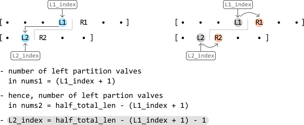
L1 ni nums1 ustida qidiramiz, bu tartiblangan massiv, shuning uchun ikkilik qidiruvdan foydalanishimiz mumkin.
Qidiruv maydonini qanday toraytirishni aniqlaylik. L1 ning o'rta nuqta indeksini mid deb belgilaymiz.
- Agar L1 > R2 bo'lsa, L1 kutilganidan kattaroq — uni kamaytirish kerak. O'rta nuqtani chapga siljiting.
- Agar L2 > R1 bo'lsa, R1 kutilganidan kichikroq — uni oshirish kerak. O'rta nuqtani o'ngga siljiting.
- Agar L1 ≤ R2 va L2 ≤ R1 bo'lsa, to'g'ri kesim topildi:
Qidiruv maydonini optimallashtirish Kichik optimallashtirish — nums1 ni qisqaroq massiv bo'lishini ta'minlash, chunki biz faqat uning ustida ikkilik qidiruv olib boramiz.
O'rta qiymatni qaytarish Ikkilik qidiruv to'g'ri kesimni topgandan so'ng, o'rta qiymatni hisoblashimiz kerak.
![Image represents a visual explanation of a merge sort algorithm step. Two arrays, `[0 2 5 6 8]` and `[0 3 7]`, are shown, with their elements visually separated by a vertical line. Light blue circles highlight the numbers 2 and 3 in the respective arrays, indicating these are the largest element in the left array and the smallest element in the right array, respectively. A curved arrow points from the 3 to indicate that it's the smallest element on the right, and another curved arrow points to the 3 from the left to indicate that it's the largest element on the left. An orange circle highlights the number 5 in the right array, indicating it's the smallest element in that array. Below, a merged array `[0 1 2 3 5 6 7 8]` is displayed, showing the result of merging the two input arrays in sorted order. The numbers 1 and 2 are implicitly understood to be part of the merged array, as they are the next smallest elements after 0. The diagram illustrates the process of selecting the smallest element from the right array and the largest element from the left array during the merging phase of the merge sort.](https://bytebytego.com/images/courses/coding-patterns/binary-search/find-the-median-from-two-sorted-arrays/image-06-05-12-EH53SBS2.svg?dpl=dpl_Gs7zfM6MUzjTBjcjps1LqXtb9QmD)
Shunday qilib, o'rta qiymatni qaytarish uchun bu ikki qiymat yig'indisini 2 ga bo'lish kifoya.
Umumiy uzunlik toq bo'lsa nima bo'ladi? Asosiy farq shundaki, o'ng yarmi bir qiymat ko'proq bo'ladi.
![Image represents a demonstration of merging two sorted arrays. The top line shows an array named `nums1` containing the integer elements [0, 2, 5, 6, 8]. The second line displays another array, `nums2`, with elements [1, 3, 7, 9]. Below these, labeled 'merged array:', is the result of merging `nums1` and `nums2` into a single sorted array: [0, 1, 2, 3, 5, 6, 7, 8, 9]. The elements from `nums1` are shown in black, while elements from `nums2` are displayed in light blue and orange, illustrating their origin within the merged array. There are no URLs or parameters present; the image solely depicts the data structures and the outcome of the merging operation.](https://bytebytego.com/images/courses/coding-patterns/binary-search/find-the-median-from-two-sorted-arrays/image-06-05-13-LP2EV7RN.svg?dpl=dpl_Gs7zfM6MUzjTBjcjps1LqXtb9QmD)
Yuqoridagi diagramma o'ng yarmida bir qiymat ortiqcha ekanligini ko'rsatadi. Bu holda o'rta qiymat bitta bo'ladi.
![Image represents a partially merged array visualized during a merge sort algorithm. The text 'merged array:' labels a numerical array represented within square brackets `[]`. The array contains elements colored in two different colors: `0`, `1`, `2`, and `3` are displayed in cyan, while `5`, `6`, `7`, `8`, and `9` are in orange. A vertical bar `|` and brackets `[]` highlight the number `5` within the orange section. An orange curved arrow points from the text 'start of right half' to the highlighted `5`, indicating that this element represents the beginning of the right half of an array that is being merged with a left half (represented by the cyan numbers). The overall image illustrates a step in the merge sort process where the algorithm is combining sorted sub-arrays.](https://bytebytego.com/images/courses/coding-patterns/binary-search/find-the-median-from-two-sorted-arrays/image-06-05-14-J2LJI2YA.svg?dpl=dpl_Gs7zfM6MUzjTBjcjps1LqXtb9QmD)
Shunday qilib, ikkilik qidiruv to'g'ri kesimni topgandan so'ng, chap bo'linmaning eng katta qiymatini qaytarish mumkin.
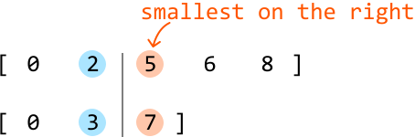
Amalga oshirish
from typing import List

def find_the_median_from_two_sorted_arrays(nums1: List[int], nums2: List[int]) -> float:
    # Optimization: ensure 'nums1' is the smaller array.
    if len(nums2) < len(nums1):
        nums1, nums2 = nums2, nums1
    m, n = len(nums1), len(nums2)
    half_total_len = (m + n) // 2
    left, right = 0, m - 1
    # A median always exists in a non-empty array, so continue binary search until
    # it's found.
    while True:
        L1_index = (left + right) // 2
        L2_index = half_total_len - (L1_index + 1) - 1
        # Set to -infinity or +infinity if out of bounds.
        L1 = float('-inf') if L1_index < 0 else nums1[L1_index]
        R1 = float('inf') if L1_index >= m - 1 else nums1[L1_index + 1]
        L2 = float('-inf') if L2_index < 0 else nums2[L2_index]
        R2 = float('inf') if L2_index >= n - 1 else nums2[L2_index + 1]
        # If 'L1 > R2', then 'L1' is too far to the right. Narrow the search space
        # toward the left.
        if L1 > R2:
            right = L1_index - 1
        # If 'L2 > R1', then 'L1' is too far to the left. Narrow the search space
        # toward the right.
        elif L2 > R1:
            left = L1_index + 1
        # If both 'L1' and 'L2' are less than or equal to both 'R1' and 'R2', we
        # found the correct slice.
        else:
            if (m + n) % 2 == 0:
                return (max(L1, L2) + min(R1, R2)) / 2.0
            else:
                return min(R1, R2)
Murakkablik tahlili
Vaqt murakkabligi: find_the_median_from_two_sorted_arrays funksiyasining vaqt murakkabligi O(log(min(m, n))) — eng qisqa massiv ustida ikkilik qidiruv amalga oshiriladi.
Xotira murakkabligi: Xotira murakkabligi O(1).
Eslatma: bu tushuntirishda ikki o'rta qiymat "median qiymatlar" deb ataladi, soddalik uchun.
Matritsa Qidiruvi
Matritsa Qidiruvi
Matritisada target qiymat mavjudligini aniqlang. Matritisaning har bir qatori o'smaydigan tartibda tartiblangan.
Misol:
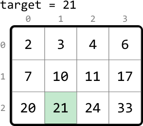
Output: True
Fikrlash tarzi
Bu masalaning oddiy yechimi — maqsad qiymatni topguncha matritsani chiziqli ravishda ko'rib chiqish. Bu O(m*n) vaqt murakkabligiga olib keladi.
Asosiy kuzatuv: berilgan qatordagi barcha qiymatlar oldingi qatordagi barcha qiymatlardan katta yoki teng. Bu matritsaning tartiblangan xususiyatini bildiradi.
![Image represents a data transformation process visualized using a matrix and arrows. A 3x4 matrix is shown, with rows labeled 0, 1, and 2, and columns labeled 0, 1, 2, and 3. Each cell in the matrix contains a numerical value (2, 3, 4, 6, 7, 10, 11, 17, 20, 21, 24, 33). Light orange arrows indicate data flow. Two arrows originate from the top-left corner of the matrix, one from row 0 and one from row 1, pointing downwards to a horizontal array below the matrix. This array displays the values from the first two rows of the matrix, concatenated horizontally ([2, 3, 4, 6, 7, 10, 11, 17]). A third arrow originates from the right side of the matrix, pointing downwards to another horizontal array, which displays the values from the last row of the matrix, concatenated horizontally ([20, 21, 24, 33]). The final output is a single horizontal array containing all the values from the matrix, arranged sequentially.](https://bytebytego.com/images/courses/coding-patterns/binary-search/matrix-search/image-06-06-1-VM2AAQRO.svg?dpl=dpl_Gs7zfM6MUzjTBjcjps1LqXtb9QmD)
Agar bu matritsani bitta tartiblangan massivga tekislashtira olsak, ikkilik qidiruv ishlatishimiz mumkin.
Tekislangan massivning indekslarini matritsadagi tegishli kataklarga moslashtirailik.
Bu indeks moslashuvi matritsaning elementlariga tartiblangan massiv sifatida kirishning yo'lini beradi.
Matritsaning har bir qatorining mapped indekslarini ko'rib chiqaylik:
- 0-qator 0-indeksdan boshlanadi.
- 1-qator n-indeksdan boshlanadi.
- 2-qator 2n-indeksdan boshlanadi.
Yuqoridagi kuzatuvlardan bir naqsh ko'rinadi: har qanday r qator uchun qatorning birinchi katagi r*n indeksiga to'g'ri keladi.
Ustun qiymatini c ni ham hisobga olsak, har qanday (r, c) katagi i = r*n + c ga to'g'ri keladi degan xulosaga kelamiz.
2D matritsaning 1D tekislangan massivga qanday moslashishini tushunganimizdan so'ng, teskari formulalarni yozamiz:
- r = i // n
- c = i % n
Bularni quyida qanday olinganligini ko'rishimiz mumkin:
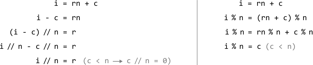
Endi bu formulalar mavjud, maqsadni topish uchun ikkilik qidiruvdan foydalanaylik.
Ikkilik qidiruv Qidiruv maydonini aniqlash uchun tekislangan massivning birinchi va oxirgi indekslariga ehtiyojimiz bor.
Qidiruv maydonini qanday toraytirishni aniqlash uchun quyidagi misol matritsasini ko'rib chiqaylik.
mid ni mid = (left + right) // 2 formulasi bilan hisoblab, keyin tegishli (r, c) katakka o'tib, qiymatni maqsad bilan taqqoslaymiz.
![Image represents a visual explanation of a search algorithm within a 4x4 matrix. The top shows 'target = 21,' indicating the value being searched for. A 4x4 matrix is displayed below, with each cell containing a number and its row and column index shown as subscripts. The matrix is labeled with 'left', 'mid', and 'right' indicating index pointers. The 'mid' pointer highlights the value 10 at row 1, column 1. To the right, calculations are shown: 'r = mid // n' (integer division of 'mid' by 4, resulting in 1) and 'c = mid % n' (modulo operation of 'mid' by 4, resulting in 1). This determines the row (r=1) and column (c=1) of the element to check. The condition 'matrix[r][c] < target' (10 < 21) is shown, indicating that the element at row 1, column 1 is less than the target. Finally, the consequence 'left = mid + 1' is shown, suggesting the algorithm updates the 'left' pointer based on the comparison result. The highlighted cell (21) shows the target value found in the matrix.](https://bytebytego.com/images/courses/coding-patterns/binary-search/matrix-search/image-06-06-5-DMLIZWBT.svg?dpl=dpl_Gs7zfM6MUzjTBjcjps1LqXtb9QmD)
Yangi o'rta qiymat ham maqsaddan kichik, shuning uchun qidiruv maydonini yana toraytiramiz.
![Image represents a visual explanation of a search algorithm within a 4x4 matrix. The top shows 'target = 21,' indicating the value being searched for. A 4x4 matrix is displayed below, with rows labeled 0, 1, 2 and columns labeled 0, 1, 2, 3. Each cell contains a number, and the cell containing 20 is labeled 'mid' (in cyan), the cell containing 11 is labeled 'left' (in orange), and the cell containing 33 is labeled 'right' (in orange). To the right, a separate box details the calculation process: 'r = mid // n' (integer division of mid by n, where mid is 8 and n is 4, resulting in r=2) and 'c = mid % n' (modulo operation of mid by n, resulting in c=0). The line 'matrix[r][c] < target' indicates a comparison between the value at matrix position [2][0] (which is 20) and the target value (21). The result of this comparison (20 < 21) leads to the assignment 'left = mid + 1,' implying an adjustment of the search range based on the comparison. The overall diagram illustrates a step in a binary search or similar algorithm applied to a 2D array.](https://bytebytego.com/images/courses/coding-patterns/binary-search/matrix-search/image-06-06-7-L47BY2QA.svg?dpl=dpl_Gs7zfM6MUzjTBjcjps1LqXtb9QmD)
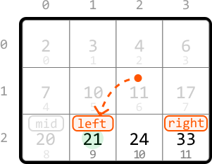
O'rta qiymat endi maqsaddan katta, ya'ni maqsad chapda joylashgan.
![Image represents a visual explanation of a search algorithm within a 4x4 matrix. The top shows 'target = 21,' indicating the value being searched for. A 4x4 matrix is displayed below, with each cell containing a number and its row and column indices subtly indicated. The matrix's rows are indexed 0, 1, and 2, and columns are indexed 0, 1, 2, and 3. The number 21 is highlighted within the matrix, labeled 'left,' indicating its position in the search. To its right is the number 24, labeled 'mid,' and to its further right is 33, labeled 'right.' These labels suggest a binary search-like approach. A separate box to the right details the calculation process: 'r = mid // n' and 'c = mid % n' calculate the row (r) and column (c) indices of the 'mid' element (24 in this case), where 'mid' is 10 (its index in a flattened array), 'n' is 4 (the number of columns). The calculations show r = 2 and c = 2. Finally, 'matrix[r][c] > target → right = mid - 1' indicates that if the value at matrix[2][2] (which is 24) is greater than the target (21), the right boundary of the search is updated to 'mid - 1', effectively narrowing the search space.](https://bytebytego.com/images/courses/coding-patterns/binary-search/matrix-search/image-06-06-9-D5J3SWTK.svg?dpl=dpl_Gs7zfM6MUzjTBjcjps1LqXtb9QmD)
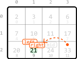
Endi o'rta nuqta maqsadga teng, shuning uchun qidiruvni tugatkanimizni bildirish uchun true qaytaramiz.
![Image represents a visual explanation of a search algorithm within a matrix. A 3x4 matrix is shown, with each cell containing a number and its index (row, column) subtly displayed below. The top row displays column indices (0, 1, 2, 3), and the leftmost column displays row indices (0, 1, 2). The number 21 is highlighted within the matrix at index (2,1), indicating a 'mid' value. To the right, a separate box details the calculation: `r = mid // n` (integer division of `mid` (9) by `n` (4), resulting in `r = 2`) and `c = mid % n` (modulo operation of `mid` (9) by `n` (4), resulting in `c = 1`). This calculation determines the row (`r`) and column (`c`) indices of the element being checked. Finally, the condition `matrix[r][c] == target` is shown, indicating that if the element at the calculated index (`matrix[2][1]`) equals the `target` value (21), the function returns `True`. The overall diagram illustrates how a search algorithm might locate a target value within a matrix using integer division and modulo operations to determine the index.](https://bytebytego.com/images/courses/coding-patterns/binary-search/matrix-search/image-06-06-11-243Y7DAT.svg?dpl=dpl_Gs7zfM6MUzjTBjcjps1LqXtb9QmD)
Chiqish sharti while left ≤ right bo'lishi kerak, chunki faqat bitta elementli qidiruv maydonini ham ko'rib chiqishimiz kerak.
Amalga oshirish
from typing import List

def matrix_search(matrix: List[List[int]], target: int) -> bool:
    m, n = len(matrix), len(matrix[0])
    left, right = 0, m * n - 1
    # Perform binary search to find the target.
    while left <= right:
        mid = (left + right) // 2
        r, c = mid // n, mid % n
        if matrix[r][c] == target:
            return True
        elif matrix[r][c] > target:
            right = mid - 1
        else:
            left = mid + 1
    return False
Murakkablik tahlili
Vaqt murakkabligi: matrix_search ning vaqt murakkabligi O(log(m*n)) — tekislangan massivda ikkilik qidiruv amalga oshiriladi.
Xotira murakkabligi: Xotira murakkabligi O(1).
Massivda Mahalliy Maksimum
Massivda Mahalliy Maksimum
Mahalliy maksimum — ikkala yaqin qo'shnilaridan ham katta qiymat. Massivda ixtiyoriy mahalliy maksimumni qaytaring.
Misol:
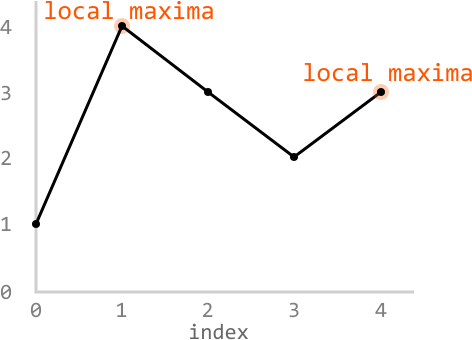
Input: nums = [1, 4, 3, 2, 3]
Output: 1 # index 4 is also acceptable
Cheklovlar:
- Massivda ikkita qo'shni element teng bo'lmaydi.
Fikrlash tarzi
Bu masalani hal qilishning oddiy usuli — har bir elementni iteratsiya orqali ko'rib chiqib, mahalliy maksimumni chiziqli ravishda qidirish. Bu O(n) vaqt oladi.
E'tiborga olish kerak bo'lgan birinchi narsa — bu massivda teng qo'shni elementlar yo'q, shuning uchun massivda har doim kamida bitta mahalliy maksimum mavjud.
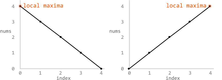
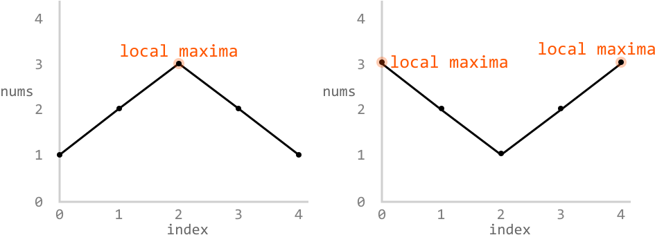
Faraz qilaylik, massivning tasodifiy i indeksidamiz. Qiziqarli kuzatuv: agar i va i+1 nuqtalar ko'tariluvchi qiyalikni hosil qilsa, u holda mahalliy maksimum o'ng tomonda joylashgan.
![Image represents a diagram illustrating a condition within a coding pattern, likely related to finding local maxima in an array. Two orange circles represent array indices 'i' and 'i+1', with downward-pointing orange arrows indicating access to the corresponding array elements `nums[i]` and `nums[i+1]`. A thick black line connects the circle representing 'i' to a black dot representing an intermediate state. A dashed line extends from this dot, suggesting a continuation. An orange arrow points from 'i+1' to this black dot. The text `nums[i] < nums[i+1]` indicates a comparison between the values at these indices. A rightward arrow follows this comparison, leading to the text 'local maxima somewhere to the right of i,' implying that if the condition `nums[i] < nums[i+1]` is true, a local maximum is expected to exist at some index greater than 'i'. The overall diagram visually represents the logic flow of checking for an increasing trend in the array to potentially identify a local maximum.](https://bytebytego.com/images/courses/coding-patterns/binary-search/local-maxima-in-array/image-06-07-3-2BDSJVMT.svg?dpl=dpl_Gs7zfM6MUzjTBjcjps1LqXtb9QmD)
Aksincha, agar i va i+1 nuqtalar tushuvchi qiyalikni hosil qilsa, mahalliy maksimum chap tomonda joylashgan.
![Image represents a diagram illustrating a condition for identifying local maxima within a numerical sequence represented by the array `nums`. The diagram features two nodes, one colored orange and the other black, connected by a solid black arrow pointing from the orange node to the black node. Above the orange node, a downward-pointing orange arrow labeled 'i' indicates an index `i` in the `nums` array. Similarly, a downward-pointing orange arrow labeled 'i+1' points to the black node, representing the next index `i+1`. A dashed line extends from a point slightly to the left and above the orange node, suggesting a continuation of the sequence before index `i`. The core logic is expressed as `nums[i] > nums[i+1]`, indicating that if the value at index `i` is greater than the value at index `i+1`, then either a local maximum exists somewhere to the left of index `i`, or the value at `nums[i]` itself is a local maximum. The text to the right of the inequality explains these two possible outcomes.](https://bytebytego.com/images/courses/coding-patterns/binary-search/local-maxima-in-array/image-06-07-4-OVOZ7QYW.svg?dpl=dpl_Gs7zfM6MUzjTBjcjps1LqXtb9QmD)
Mahalliy maksimum chap yoki o'ngda ekanligini bilganimizdan so'ng, qidiruv maydonini mos tomoniga toraytirish mumkin.
Ikkilik qidiruv Qidiruv maydonini aniqlash uchun massivning birinchi va oxirgi indekslaridan foydalanamiz. Mahalliy maksimum istalgan joyda bo'lishi mumkin.
Qidiruv maydonini toraytirish uchun quyidagi misoldan foydalanamiz, left = 0, right = n-1 bilan boshlaymiz.
![Image represents a line graph illustrating a numerical array. The horizontal axis is labeled 'index' and ranges from 0 to 6. The vertical axis is labeled 'nums' and ranges from 0 to 4. A black line connects data points representing the values of an array [0, 1, 4, 2, 1, 2, 3], where each number corresponds to its index. The array is displayed above the graph. Two orange vertical lines highlight the leftmost (index 0, value 0) and rightmost (index 6, value 3) elements of the array. Above these lines, orange rectangular boxes labeled 'left' and 'right' respectively, indicate the boundaries. The area under the line graph is filled with a light peach color.](https://bytebytego.com/images/courses/coding-patterns/binary-search/local-maxima-in-array/image-06-07-5-KNRFX744.svg?dpl=dpl_Gs7zfM6MUzjTBjcjps1LqXtb9QmD)
O'rta nuqta dastlab 3-indeksga qo'yiladi, u o'ng qo'shnisi bilan tushuvchi qiyalik hosil qiladi. Demak, mahalliy maksimum 3-indeksning chap tomonida.
![Image represents two line graphs illustrating a coding pattern, likely a binary search algorithm. Both graphs display the same data points: `[0, 1, 4, 2, 1, 2, 3]` plotted against an index from 0 to 6. The y-axis represents the 'nums' values. In both graphs, vertical orange lines mark 'left' and 'right' boundaries, and a light-blue arrow indicates 'mid'. The left graph shows the initial state with 'left' at index 0, 'mid' at index 3, and 'right' at index 6. A shaded peach area highlights the section between 'left' and 'right'. The right graph depicts an iteration where a descending slope is detected (nums[mid] > nums[mid + 1]), resulting in 'right' being updated to the 'mid' index (index 3). A dashed orange line connects the old and new 'right' positions. A grey box in the left graph explains the condition for updating 'right' in the algorithm: `descending slope: nums[mid] > nums[mid + 1] → right = mid`. A small arrow points from this box to the right graph, indicating the application of this rule.](https://bytebytego.com/images/courses/coding-patterns/binary-search/local-maxima-in-array/image-06-07-6-SAXUDM6W.svg?dpl=dpl_Gs7zfM6MUzjTBjcjps1LqXtb9QmD)
Keyingi o'rta nuqta 1-indeksga qo'yiladi, u o'ng qo'shnisi bilan ko'tariluvchi qiyalik hosil qiladi. Demak, mahalliy maksimum o'ng tomonda.
![Image represents a visual explanation of a coding pattern, likely within a sorting or searching algorithm. The image is divided into two nearly identical parts, each showing a line graph with a series of points connected by lines. The x-axis represents an index (0-6), and the y-axis represents numerical values ('nums'). In both parts, orange vertical lines highlight sections of the graph. Above each graph, rectangular boxes labeled 'left,' 'mid,' and 'right' indicate index values (e.g., [0 1 4 2 1 2 3] in the first part) that are associated with the graph's points. Arrows point from these boxes down to their corresponding points on the graph. A dashed gray line connects the 'left' and 'right' indices in the second part, suggesting a range. A light peach-colored rectangle highlights a section of the graph between the 'left' and 'right' markers. A separate box explains the condition 'ascending slope: nums[mid] < nums[mid + 1] → left = mid + 1,' indicating that if the value at the midpoint is less than the value at the next point, the 'left' index is updated to the midpoint plus one. This suggests an iterative process of narrowing down a search range based on the slope of the line graph. The two parts likely illustrate different stages of this iterative process.](https://bytebytego.com/images/courses/coding-patterns/binary-search/local-maxima-in-array/image-06-07-7-TQDRJDPG.svg?dpl=dpl_Gs7zfM6MUzjTBjcjps1LqXtb9QmD)
Keyingi o'rta nuqta 2-indeksga qo'yiladi, u o'ng qo'shnisi bilan tushuvchi qiyalik hosil qiladi. Demak, mahalliy maksimum 2-indeksning chap tomonida yoki 2-indeksning o'zida.
![Image represents a visual explanation of a coding pattern, likely within a binary search algorithm. The image is divided into two nearly identical halves, each showing a line graph plotting a numerical array `nums` against its index. The x-axis represents the index (0 to 6), and the y-axis represents the values within the `nums` array. Both graphs depict the same data, a series of points connected by lines forming a V-shape. At the top of each half, labeled boxes indicate pointers `left`, `mid`, and `right`, initially pointing to indices 0, 2, and 3 respectively in the left half and 0, 1, and 3 in the right half. These pointers define a search window within the array. A shaded orange vertical bar highlights the `mid` index in the left graph. A gray box in the left half explains a condition: 'descending slope: nums[mid] > nums[mid + 1] → right = mid,' indicating that if the value at `mid` is greater than the value at `mid + 1`, the `right` pointer is updated to `mid`, effectively narrowing the search space. The right half likely shows the result of applying this condition, with the `right` pointer moved to index 1. The overall diagram illustrates how the algorithm iteratively refines the search range based on the slope of the data.](https://bytebytego.com/images/courses/coding-patterns/binary-search/local-maxima-in-array/image-06-07-8-6TRJFGAS.svg?dpl=dpl_Gs7zfM6MUzjTBjcjps1LqXtb9QmD)
Endi left va right ko'rsatkichlar uchrashib, 2-indeksni mahalliy maksimum sifatida topdi.
Xulosa 1-holat: O'rta nuqta o'ng qo'shnisi bilan tushuvchi qiyalik hosil qiladi — mahalliy maksimum chapda yoki o'rta nuqtaning o'zida. right = mid.
![Image represents a visual explanation of a step within a binary search algorithm, specifically illustrating a condition where the middle element is greater than the element to its right. The image is divided into two parts separated by a large right-pointing arrow. The left part shows an array `[0, 4, 3, 1, 0]` represented graphically as a line graph with the x-axis representing the index (0 to 4) and the y-axis representing the array's values (0 to 4). Vertical orange lines mark the `left` (index 0), `mid` (index 2), and `right` (index 4) pointers, with corresponding labels above the lines. A shaded peach area highlights the section of the array between `left` and `right`. A black line connects the data points, showing the array's values. The right part shows the updated state after the condition `if nums[mid] > nums[mid + 1]: right = mid;` is executed. The `right` pointer has moved from index 4 to index 2, indicated by a dashed orange line connecting the old and new positions. The graph is updated to reflect this change, with the new `right` pointer at index 2. Above both parts, a code snippet displays the condition `if nums[mid] > nums[mid + 1]: right = mid;`, which is the decision-making logic behind the pointer movement. The overall image demonstrates how the algorithm adjusts its search space based on the comparison of the middle element with its neighbor to the right.](https://bytebytego.com/images/courses/coding-patterns/binary-search/local-maxima-in-array/image-06-07-9-KWRDIDZZ.svg?dpl=dpl_Gs7zfM6MUzjTBjcjps1LqXtb9QmD)
2-holat: O'rta nuqta o'ng qo'shnisi bilan ko'tariluvchi qiyalik hosil qiladi — mahalliy maksimum o'ngda. left = mid + 1.
![Image represents a visual explanation of a coding pattern, likely within a sorting algorithm. The top shows a code snippet: `if nums[mid] < nums[mid + 1]: left = mid + 1;`, indicating a conditional statement comparing two elements of an array `nums` at indices `mid` and `mid + 1`. Below, a line graph displays an array `nums` = [0, 4, 3, 1, 0] with indices 0-4 on the x-axis and values on the y-axis. Orange vertical lines mark `left` (index 0), `mid` (index 2), and `right` (index 4), initially. A shaded peach region highlights the section between `left` and `right`. A black line connects the data points. A grey dot marks the `mid` point's value. A thick black arrow separates this from a second graph showing the array after the conditional statement's execution. In the second graph, `left` has shifted to index 3, indicated by a new orange line, while `right` remains at index 4. The peach shaded region now reflects the updated `left` and `right` boundaries. The dashed orange line connects the old and new `left` positions, visually demonstrating the shift. The second graph's line plot remains the same, but the `left` pointer's position has changed, illustrating the algorithm's step in adjusting the search space based on the comparison.](https://bytebytego.com/images/courses/coding-patterns/binary-search/local-maxima-in-array/image-06-07-10-ODBVPTGZ.svg?dpl=dpl_Gs7zfM6MUzjTBjcjps1LqXtb9QmD)
Amalga oshirish
from typing import List

def local_maxima_in_array(nums: List[int]) -> int:
    left, right = 0, len(nums) - 1
    while left < right:
        mid = (left + right) // 2
        if nums[mid] > nums[mid + 1]:
            right = mid
        else:
            left = mid + 1
    return left
Murakkablik tahlili
Vaqt murakkabligi: local_maxima_in_array ning vaqt murakkabligi O(log(n)) — har bir qadamda qidiruv maydoni yarmiga qisqaradi.
Xotira murakkabligi: Xotira murakkabligi O(1).
Og'irlikli Tasodifiy Tanlash
Og'irlikli Tasodifiy Tanlash
Har biri mos og'irlikka ega elementlar massivi berilgan, elementlarni ularning og'irliklariga mutanosib ehtimollik bilan tasodifiy tanlash funksiyasini amalga oshiring.
Boshqacha aytganda, i indeksidagi elementni tanlash ehtimoli: weights[i] / sum(weights)
Tanlangan elementning indeksini qaytaring.
Misol:
Input: weights = [3, 1, 2, 4]
Tushuntirish: sum(weights) = 10 3 ning 3/10 tanlash ehtimoli bor. 1 ning 1/10 tanlash ehtimoli bor. 2 ning 2/10 tanlash ehtimoli bor. 4 ning 4/10 tanlash ehtimoli bor.
Cheklovlar:
- Og'irliklar massivida kamida bitta element bor.
Fikrlash tarzi
To'liq bir xil tasodifiy tanlash har bir indeksning teng imkoniyatga ega ekanligini anglatadi. Ammo bu masalada har bir indeksning tanlash ehtimoli og'irligiga mutanosib bo'lishi kerak.
Bu masaladagi asosiy qiyinchilik — indeksni uning og'irligi asosida tasodifiy tanlash metodini aniqlashdir.
Faraz qilaylik, 0 va 1 indekslari uchun og'irliklar mos ravishda 1 va 4:
![Image represents a Python code snippet assigning a list of weights. The snippet shows the variable `weights` being assigned a list containing two numerical values: 1 and 4. The assignment is represented using the equals sign (`=`). The list is denoted by square brackets (`[` and `]`). The numbers 0 and 1 are faintly visible below the numbers 1 and 4 respectively, possibly indicating indices or positions within the list. There is no other information, such as URLs or parameters, present in the image. The overall structure is a simple variable assignment statement common in programming languages.](https://bytebytego.com/images/courses/coding-patterns/binary-search/weighted-random-selection/image-06-08-1-VSNFN3H5.svg?dpl=dpl_Gs7zfM6MUzjTBjcjps1LqXtb9QmD)
Bu yerda 1-indeks 4/5 ehtimol bilan tanlanishi kerak, bu 0-indeksning 1/5 ehtimolidan ancha yuqori.
![Image represents a simple illustration of weight normalization in a context likely related to machine learning or weighted averaging. The top line shows a Python-like variable assignment, `weights = [1 4]`, defining a weight vector with two elements: 1 and 4. Below, these weights are individually depicted with small downward arrows pointing to their normalized counterparts. The normalization appears to be a simple division by the sum of the weights (1+4=5). Therefore, the weight 1 is transformed into 1/5 (displayed in cyan), and the weight 4 is transformed into 4/5 (displayed in orange). The small numbers '0' and '1' above the arrows likely represent indices indicating the position of each weight within the original vector. The overall diagram visually demonstrates the process of converting a set of weights into their normalized probability distribution.](https://bytebytego.com/images/courses/coding-patterns/binary-search/weighted-random-selection/image-06-08-2-RMK2AASL.svg?dpl=dpl_Gs7zfM6MUzjTBjcjps1LqXtb9QmD)
Foydali kuzatuv: barcha ehtimollar bir xil mahrajga ega (bu sum(weights) ga teng). Shuning uchun ehtimollarni kasr sifatida ifodalash o'rniga, butun sonlardan foydalanish qulay.

Agar bu chiziqda tasodifiy son tanlasak, birinchi segmentni 1/5 ehtimol bilan, ikkinchisini 4/5 ehtimol bilan tanlaymiz.

Agar chiziqda tasodifiy son tanlasak, 0-indeksni 1/5, 1-indeksni 4/5 ehtimol bilan tanlaymiz.
Endi chiziqning qaysi sonlari qaysi indekslarga mos kelishini aniqlash usuli kerak.
Davom etishdan oldin, ushbu tushuntirishda ishlatiladigan atamalar ta'riflarini belgilab olaylik.
- "Og'irliklar" weights massividagi elementlar qiymatlarini bildiradi.
- "Indekslar" weights massivining indekslarini bildiradi.
- "Sonlar" yoki "chiziqidagi sonlar" 1 dan sum(weights) gacha bo'lgan sonlarni bildiradi.
Chiziqning qaysi sonlari qaysi indekslarga mos kelishini aniqlash Yuqorida aytganimizdek, har bir indeksning o'z segmenti bor.
![Image represents a visual depiction of weighted indexing. At the top, a list named 'weights' is defined as an array containing the integers [3, 1, 2, 4]. Below this, a horizontal bar is segmented into four color-coded sections, each labeled 'index 0,' 'index 1,' 'index 2,' and 'index 3,' respectively. The bar is further divided into numbered units from 1 to 10. Colored arrows connect the weights to the bar; a cyan arrow from the weight '3' points to the end of the 'index 0' section (at position 3), a green arrow from the weight '1' points to the end of the 'index 1' section (at position 4), an orange arrow from the weight '2' points to the end of the 'index 2' section (at position 6), and a magenta arrow from the weight '4' points to the end of the 'index 3' section (at position 8). Each arrow's length visually represents the corresponding weight value, indicating how many units each index occupies within the bar. The numbers above the arrows (0, 1, 2, 3) correspond to the index of the weight in the `weights` array.](https://bytebytego.com/images/courses/coding-patterns/binary-search/weighted-random-selection/image-06-08-5-6VJFW4JM.svg?dpl=dpl_Gs7zfM6MUzjTBjcjps1LqXtb9QmD)
Bir strategiya — hash map ishlatish. Bu hash mapda chiziqning har bir soni tegishli indeksga moslashtiriladi.
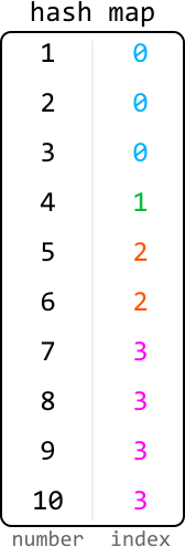
Bu metod ko'p xotira talab qiladi, chunki chiziqning har bir soni uchun kalit-qiymat juftini saqlash kerak.
Yanada samarali strategiya — har bir segmentning faqat oxirgi nuqtasini saqlash.

Tabiiy ravishda, segmentning oxirgi nuqtasi o'sha segment qayerda tugashini bildiradi. U keyingi segmentning qayerdan boshlanishini ham ko'rsatadi.
Faqat oxirgi nuqtalarni saqlash orqali har bir indeks uchun bitta qiymat — n ta qiymatni saqlash kerak.
![Image represents a visual depiction of an array, specifically a one-dimensional array or list. The array is enclosed in square brackets `[` and `]`. The array contains four elements: 3, 4, 6, and 10. These elements are displayed horizontally, separated by spaces. Below each element, in a lighter gray font, is an index indicating its position within the array. The indices start from 0 and increment sequentially: 0 for the element 3, 1 for the element 4, 2 for the element 6, and 3 for the element 10. The arrangement clearly shows the mapping between each element's value and its corresponding index within the array's structure.](https://bytebytego.com/images/courses/coding-patterns/binary-search/weighted-random-selection/image-06-08-8-2SA254H5.svg?dpl=dpl_Gs7zfM6MUzjTBjcjps1LqXtb9QmD)
Endi savol: bu oxirgi nuqtalarni qanday topamiz?
Har bir indeks segmentining oxirgi nuqtalarini olish Asosiy kuzatuv — har bir segment oldingi barcha segmentlarning oxirgi nuqtasidan keyin joylashgan.

Bu har bir oxirgi nuqta kumulyativ yig'indilar ekanligini ko'rsatadi — prefix sums massividan foydalanishimiz mumkin.

Ko'rib turganimizdek, prefix sums massivi har bir segmentning oxirgi nuqtasini saqlaydi.
Endi prefix sums massivi qanday yordam berishini ko'raylik. Tasodifiy son tanlaganimizda, u ma'lum bir segmentga to'g'ri keladi.
Qaysi sonlar qaysi indekslarga mos kelishini aniqlash uchun prefix sumsdan foydalanish 5 ni tasodifiy son sifatida tanlaganimizni faraz qilaylik:
- 5 ning o'zi ham oxirgi nuqta bo'lishi mumkin, chunki 5 o'z segmentining oxirgi nuqtasi bo'lishi mumkin.
- Yoki oxirgi nuqta 5 dan o'ngda joylashgan bo'lishi mumkin.
5 dan o'ngdagi barcha oxirgi nuqtalar orasida 5 ga eng yaqin bo'lgan uning segmentining oxirgi nuqtasidir.
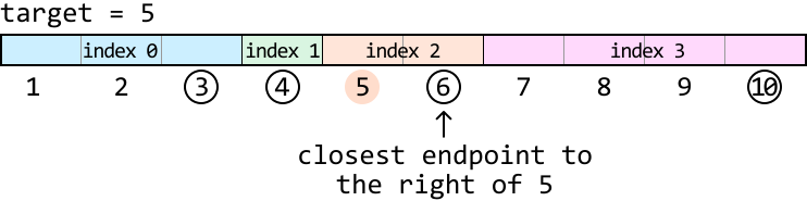
Bu shuni anglatadiki, har qanday maqsad uchun 5 dan katta yoki unga teng bo'lgan birinchi prefix summani qidiramiz.
![Image represents a depiction of prefix sums, showing an array `prefix_sums` initialized with values [3, 4, 6, 10]. The array is presented horizontally. Each element's value is displayed numerically. Below each element, a colored vertical line indicates its status: 'F' (in red) represents 'False', and 'T' (in green) represents 'True'. The first two elements (3 and 4) are marked with 'F', while the last two elements (6 and 10) are marked with 'T'. This suggests a visual representation of a boolean condition applied to the prefix sums, where the last two elements satisfy the condition and the first two do not. The arrangement visually links the numerical value of each element with its corresponding boolean status.](https://bytebytego.com/images/courses/coding-patterns/binary-search/weighted-random-selection/image-06-08-12-OL7XXR2Z.svg?dpl=dpl_Gs7zfM6MUzjTBjcjps1LqXtb9QmD)
Ko'rib turganimizdek, bu shartni qanoatlantiradigan birinchi prefix sum to'g'ri indeks bilan mos keladi.
Keling, 5 tasodifiy maqsat bilan misolimiz ustida ko'raylik. Qidiruv left = 0, right = n-1 bilan boshlanadi.
![Image represents a visual depiction of a two-pointer approach to finding a subarray with a target sum. Two orange rectangular boxes labeled 'left' and 'right' point downwards towards an array represented by `prefix_sums = [3, 4, 6, 10]`. Beneath each element of the `prefix_sums` array, its index (0, 1, 2, 3) is shown in gray. The number 6 in the `prefix_sums` array is highlighted in light green. A separate line indicates `target = 5`. The arrows from 'left' and 'right' visually suggest the movement of pointers across the `prefix_sums` array during the algorithm's execution, aiming to find a subarray whose sum equals the `target` value. The highlighted '6' likely represents a point where the algorithm might find a solution (or a relevant intermediate state), given that the difference between consecutive prefix sums could be used to determine the sum of subarrays.](https://bytebytego.com/images/courses/coding-patterns/binary-search/weighted-random-selection/image-06-08-13-PHAH5HHP.svg?dpl=dpl_Gs7zfM6MUzjTBjcjps1LqXtb9QmD)
Qidiruv maydonini toraytiramiz. Eslab qoling: maqsaddan ≥ bo'lgan eng kichik prefix summani qidiramiz.
Boshlang'ich o'rta nuqta qiymati 4, maqsad 5 dan kichik. Demak, javob o'ngda joylashgan. left = mid + 1.
![Image represents a visual depiction of a binary search algorithm's step within the context of prefix sums. The diagram shows four labeled boxes: 'left,' 'mid,' and 'right' representing index pointers, and a dashed box containing a conditional statement. 'left' and 'mid' point downwards to an array [3, 4, 6, 10] with indices 0, 1, 2, and 3 respectively displayed below each element. 'right' also points downwards to the same array. Below the array, 'target = 5' is specified. The dashed box displays the condition 'prefix_sums[mid] < target,' which evaluates whether the prefix sum at the 'mid' index is less than the target value (5). If true, as indicated by the arrow, the 'left' pointer is updated to 'mid + 1,' effectively narrowing the search space in a binary search fashion. The light blue box around 'mid' and the blue arrow visually emphasize the current 'mid' index and its role in the conditional statement.](https://bytebytego.com/images/courses/coding-patterns/binary-search/weighted-random-selection/image-06-08-14-L7WTQG3L.svg?dpl=dpl_Gs7zfM6MUzjTBjcjps1LqXtb9QmD)
![Image represents a visual depiction of a binary search algorithm's step. A sorted array `[3, 4, 6, 10]` is shown with indices 0, 1, 2, and 3 labeled below each element. A light gray rectangle labeled 'mid' points to the element '4' at index 1. An orange rectangle labeled 'left' points to the element '6' at index 2. A dark gray rectangle labeled 'right' points to the element '10' at index 3. A dashed orange line connects the 'mid' label to the element '3' at index 0, indicating a comparison. A solid orange arrow points from 'left' to '6', showing the selection of the left subarray. A solid dark gray arrow points from 'right' to '10', showing the selection of the right subarray. The arrangement visually demonstrates the partitioning of the array during a binary search iteration, with the 'mid' element acting as the pivot for comparison and subsequent subarray selection.](https://bytebytego.com/images/courses/coding-patterns/binary-search/weighted-random-selection/image-06-08-15-JMX3OC5G.svg?dpl=dpl_Gs7zfM6MUzjTBjcjps1LqXtb9QmD)
O'rta nuqta qiymati endi 6, maqsaddan katta. Bu o'rta nuqta shartni qanoatlantiradi — uni potentsial javob sifatida belgilaymiz. right = mid - 1.
![Image represents a visual depiction of a binary search algorithm step within a coding pattern context. The top shows three labeled boxes: 'left,' 'mid' (highlighted in cyan), and 'right.' Arrows point downwards from 'left' and 'right' to the array [3, 4, 6, 10], indicating index positions 0, 2, and 3 respectively. The 'mid' box points to the element '6' at index 2. Below the array, 'target = 5' is specified. A dashed box to the right shows a conditional statement: 'prefix_sums[mid] ≥ target,' which evaluates whether the prefix sum at the midpoint (6 in this case) is greater than or equal to the target (5). A right-pointing arrow from this condition leads to the assignment 'right = mid,' indicating that if the condition is true, the right boundary of the search space is updated to the midpoint. The overall diagram illustrates a single iteration of a binary search, where the algorithm checks if the prefix sum at the midpoint meets or exceeds the target value to refine the search range.](https://bytebytego.com/images/courses/coding-patterns/binary-search/weighted-random-selection/image-06-08-16-FXC252RT.svg?dpl=dpl_Gs7zfM6MUzjTBjcjps1LqXtb9QmD)
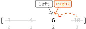
Endi left va right ko'rsatkichlar uchrashdi, 1-indeksni javob sifatida topdi.
![Image represents a diagram illustrating a coding pattern, possibly related to binary search or a similar algorithm. At the top, two orange rectangular boxes labeled 'left' and 'right' are shown, with downward-pointing arrows indicating data flow. Below, a horizontally oriented array or list is depicted, showing the elements [3, 4, 6, 10] with their indices [0, 1, 2, 3] displayed underneath. The 'left' and 'right' labels appear to represent pointers or indices into this array. The arrows from 'left' and 'right' point to the element '6' in the array, suggesting that these pointers are converging on a specific element. To the right, a light gray, dashed-line rectangle contains the conditional statement 'left == right' followed by a right-pointing arrow and the action 'return left'. This indicates that if the left and right pointers are equal, the algorithm returns the value at the left pointer's index. The overall diagram visualizes a search or comparison process where two pointers move towards each other until they meet, at which point a result is returned.](https://bytebytego.com/images/courses/coding-patterns/binary-search/weighted-random-selection/image-06-08-18-WPLT55QP.svg?dpl=dpl_Gs7zfM6MUzjTBjcjps1LqXtb9QmD)
Amalga oshirish
from typing import List
import random

class WeightedRandomSelection:
    def __init__(self, weights: List[int]):
        self.prefix_sums = [weights[0]]
        for i in range(1, len(weights)):
            self.prefix_sums.append(self.prefix_sums[-1] + weights[i])

    def select(self) -> int:
        # Pick a random target between 1 and the largest endpoint on the number
        # line.
        target = random.randint(1, self.prefix_sums[-1])
        left, right = 0, len(self.prefix_sums) - 1
        # Perform lower-bound binary search to find which endpoint (i.e., prefix
        # sum value) corresponds to the target.
        while left < right:
            mid = (left + right) // 2
            if self.prefix_sums[mid] < target:
                left = mid + 1
            else:
                right = mid
        return left
Murakkablik tahlili
Vaqt murakkabligi: konstruktorning vaqt murakkabligi O(n) — prefix sums massivini hisoblash uchun. pick funksiyasining vaqt murakkabligi O(log(n)) — ikkilik qidiruv.
Xotira murakkabligi: konstruktorning xotira murakkabligi O(n) — prefix sums massivini saqlash uchun. pick funksiyasining xotira murakkabligi O(1).
Stack
Stack ga Kirish
Stack ga Kirish
Fikrlash tarzi
Plastinkalar uyumini tasavvur qiling. Siz faqat uyumning tepasiga yangi plastinka qo'shishingiz mumkin va kerak bo'lganda faqat tepadan olishingiz mumkin.
Bu analogiya Stack ma'lumotlar tuzilmasining mohiyatini to'liq ifodalaydi. Tepaga plastinka qo'shish va tepadan olish — stack operatsiyalari:
- Push (elementni stackning tepasiga qo'shadi).
- Pop (stackning tepasidagi elementni olib qaytaradi).
LIFO (Last-In-First-Out) Stack LIFO tamoyiliga amal qiladi — eng so'nggi qo'shilgan element birinchi bo'lib chiqariladi.
- Ichma-ich tuzilmalarni qayta ishlash: Stack ichma-ich tuzilmalarni tahlil qilish yoki tekshirishda yaxshi variant.
- Teskari tartib: Stack ga push qilingan elementlar pop bilan teskari tartibda chiqariladi.
- Rekursiyani almashtirish: Rekursiv algoritmlar chaqiruv stackidan foydalanadi. Ba'zan stackdan explicit foydalanib, rekursiyani iterativ usulga almashtirish mumkin.
Yuqoridagi ilovalarning ba'zi misollari ushbu bobda ko'rib chiqilgan.
Quyida umumiy stack operatsiyalarining vaqt murakkabligi tavsifi keltirilgan:
| Operation | Worst case | Description |
|---|---|---|
| Push | Adds an element to the top of the stack. | |
| Pop | Removes and returns the element at the top of the stack. | |
| Peek | Returns the element at the top of the stack without removing it. | |
| IsEmpty | Checks if the stack is empty. |
Haqiqiy Dunyo Misoli
Funksiya chaqiruvlarini boshqarish: Stack ning umumiy haqiqiy dunyo misoli — funksiya chaqiruvlarini boshqarishdir.
Funksiya chaqirilganda, dastur funksiya holatini (parametrlar, lokal o'zgaruvchilar va qaytish manzili bilan birga) chaqiruv stackiga push qiladi.
Bob Mazmuni
Ushbu bob turli xil masalalarni ko'rib chiqadi va stackdan qanday foydalanishni batafsil tushuntiradi.
To'g'ri Qavs Ifodasi
To'g'ri Qavs Ifodasi
Qavslarni ifodalovchi matn berilgan bo'lib, u '(', ')', '[', ']', '{', '}' belgilarini o'z ichiga oladi. Agar qavs ketma-ketligi to'g'ri bo'lsa, true, aks holda false qaytaring.
Qavs ketma-ketligi to'g'ri hisoblanadi: har bir ochuvchi qavs mos yopuvchi qavs bilan yopilgan va qavslar to'g'ri tartibda yopilgan.
-misol:
Input: s = '([]{})'
Output: True
-misol:
Input: s = '([]{)}'
Output: False
Tushuntirish: '(' qavsi ichidagi '{' qavsidan oldin yopilgan.
Fikrlash tarzi
Dastlabki kuzatuv: har bir qavs turi uchun ochuvchi va yopuvchi qavslar soni teng bo'lishi kerak.
"()" matnini ko'rib chiqing. Birinchi qavs ochuvchi, ikkinchi qavs yopuvchi va birinchisini to'g'ri yopadi.
"[(])" matnini ko'rib chiqing. 1-indeksga yetganimizda, ikkita ochuvchi qavs yopilishini kutamiz. Qaysi biri birinchi yopilishi kerak?
![Image represents a comparison of two scenarios illustrating parenthesis matching in a coding context. The left side depicts a correctly matched sequence, showing the text 'most recent parenthesis waiting to be closed' above a gray downward-pointing arrow. This arrow points to a sequence of parentheses: `[(])`, indexed 0 to 3 from left to right. The closing parenthesis at index 3 correctly matches the opening parenthesis at index 1, indicating proper nesting. In contrast, the right side shows an incorrectly matched sequence. The text 'does not close most recent parenthesis' (in red) is positioned above a red downward-pointing arrow, which points to a similar sequence `[(])`, also indexed 0 to 3. However, here the closing parenthesis at index 3 does *not* match the most recent opening parenthesis (at index 1), highlighting an error in parenthesis matching. Both sides use the same parenthesis characters and indexing to facilitate a direct comparison of correct versus incorrect parenthesis closure.](https://bytebytego.com/images/courses/coding-patterns/stacks/valid-parenthesis-expression/image-07-01-2-HRJ6OOKR.svg?dpl=dpl_Gs7zfM6MUzjTBjcjps1LqXtb9QmD)
Asosiy kuzatuv: eng so'nggi uchragan ochuvchi qavs birinchi bo'lib yopilishi kerak — bu LIFO tamoyili.
Stack Yuqori darajadagi strategiya:
- Uchragan har bir ochuvchi qavsni stackga qo'shamiz. Shunday qilib, eng so'nggi qavs doim tepada turadi.
- Yopuvchi qavs uchraganda, u stackning tepasidagi ochuvchi qavsni yopa oladimi yoki yo'qligini tekshiramiz.
Keling, bu strategiya misolda qanday ishlashini ko'raylik:
![Image represents a sequence of six distinct symbols, arranged horizontally from left to right with spaces between them. The symbols are: an opening parenthesis `(`, an opening square bracket `[`, a closing square bracket `]`, an opening curly brace `{`, a closing parenthesis `)`, and a closing curly brace `}`. There are no connections or information flow depicted between the symbols; they are simply presented as individual, independent elements. No labels, text, URLs, or parameters are present within the image. The image likely illustrates the different types of grouping symbols used in programming languages or mathematical notation.](https://bytebytego.com/images/courses/coding-patterns/stacks/valid-parenthesis-expression/image-07-01-3-C47V3JIY.svg?dpl=dpl_Gs7zfM6MUzjTBjcjps1LqXtb9QmD)
Har bir ochuvchi qavs uchun uni stackga push qilamiz:
![Image represents a visual explanation of a stack data structure used for parenthesis matching. On the left, a sequence of opening and closing parentheses, brackets, and braces – `( [ ] { } )` – is shown, with an orange square containing an 'i' and a downward arrow pointing to the sequence, suggesting input. On the right, a diagram depicts a stack labeled 'stack' with a 'top' indicator. A light-grey 'top:' label points to the top of the stack, which is currently empty. A light-blue arrow labeled 'push (' indicates that the opening parenthesis '(' is being pushed onto the stack, implying that the algorithm is processing the input sequence from left to right and using the stack to keep track of opening delimiters. The overall image illustrates the initial step of a parenthesis matching algorithm using a stack.](https://bytebytego.com/images/courses/coding-patterns/stacks/valid-parenthesis-expression/image-07-01-4-VOQ7XKKN.svg?dpl=dpl_Gs7zfM6MUzjTBjcjps1LqXtb9QmD)
![Image represents a visual explanation of a stack data structure used in coding, specifically demonstrating a push operation. On the left, a sequence of opening and closing parentheses, brackets, and braces: `( [ ] { ) }` is shown. An orange square containing an 'i' symbol, suggesting input, points downwards with an arrow towards the '[' bracket, indicating the element being processed. On the right, a diagram depicts a stack labeled 'stack' with a 'top' pointer. The stack currently contains an opening parenthesis '('. A light-blue arrow labeled 'push [' shows the '[' bracket being added to the top of the stack, illustrating the 'push' operation where a new element is added to the top of the stack. The arrangement visually explains how an input element is added to the stack, modifying its contents and updating the top pointer.](https://bytebytego.com/images/courses/coding-patterns/stacks/valid-parenthesis-expression/image-07-01-5-W64UEXYI.svg?dpl=dpl_Gs7zfM6MUzjTBjcjps1LqXtb9QmD)
Keyin yopuvchi qavs uchraymiz. Uni stackning tepasidagi ochuvchi qavs bilan taqqoslaymiz.
![Image represents a visual explanation of a stack data structure used for parenthesis matching. On the left, a sequence of opening and closing parentheses, brackets, and braces — `(`, `[`, `]`, `{`, `)` — is shown. An orange square labeled 'i' points downwards, indicating an input stream of these characters. To the right, a stack is depicted as a container labeled 'stack' with a 'top' pointer indicating the top element. Inside the stack, an opening bracket '[' is present. A purple arrow labeled 'pop' extends from the top of the stack to a light gray dashed box containing the text ''[' is closed by ']':', illustrating that the top element '[' is being popped from the stack, implying a matching closing bracket ']' is expected in the input stream to maintain balanced parentheses. The diagram demonstrates how a stack is used to verify the correct pairing of opening and closing delimiters in a given input string.](https://bytebytego.com/images/courses/coding-patterns/stacks/valid-parenthesis-expression/image-07-01-6-QKVFAV54.svg?dpl=dpl_Gs7zfM6MUzjTBjcjps1LqXtb9QmD)
Keyingi belgi ochuvchi qavs — uni stackning tepasiga push qilamiz:
![Image represents a visual explanation of a stack data structure and its 'push' operation. The left side shows a sequence of opening and closing brackets and braces: '(', '[', ']', '{', ')', '}'. A downward-pointing orange arrow with a small orange square containing an 'i' (likely indicating information or instruction) points to the '{' character. This suggests the '{' is the next element to be processed. The right side depicts a stack labeled 'stack' with its contents shown as '{' and '('; the label 'top:' indicates the top of the stack. A light-blue arrow labeled 'push { ' points from the right to the stack, illustrating the 'push' operation where the '{' character is being added to the top of the stack. The overall diagram demonstrates how a character ('{') is pushed onto a stack, which is a Last-In, First-Out (LIFO) data structure.](https://bytebytego.com/images/courses/coding-patterns/stacks/valid-parenthesis-expression/image-07-01-7-2PAD6WHB.svg?dpl=dpl_Gs7zfM6MUzjTBjcjps1LqXtb9QmD)
Keyingi belgi ')' — u stackning tepasidagi ochuvchi qavsni yopa olmaydi, shuning uchun false qaytaramiz.
![Image represents a visual explanation of a stack-based approach to validating balanced parentheses in a code snippet. On the left, a sequence of opening and closing parentheses, brackets, and braces (`(`, `[`, `{`, `)`, `]`, `}`) is shown. An orange arrow with an 'i' icon points downwards towards the curly brace '{' and closing parenthesis ')'. To the right, a diagram depicts a stack data structure labeled 'stack,' with the characters '{' and '(' currently inside it, indicating that these opening brackets have been pushed onto the stack. The label 'top:' points to the top of the stack, which is '{'. A light gray dashed-line box contains pseudocode: `'{' is not closed by ')': return False`, illustrating a scenario where an opening curly brace '{' is encountered, but its corresponding closing brace '}' is not found before a closing parenthesis ')', resulting in a `False` return value, indicating unbalanced parentheses. The overall image demonstrates how a stack can be used to track opening brackets and check for proper closing counterparts during code validation.](https://bytebytego.com/images/courses/coding-patterns/stacks/valid-parenthesis-expression/image-07-01-8-WBRUNMV4.svg?dpl=dpl_Gs7zfM6MUzjTBjcjps1LqXtb9QmD)
Agar butun matnni false qaytarmasdan o'tsak, barcha qavslar muvaffaqiyatli yopilgan.
Chekka holat: ortiqcha ochuvchi qavslar Faqat yopuvchi qavslarda noto'g'rilikni tekshiramiz, shuning uchun barcha ochuvchi qavslar yopilganligini ham tekshirish kerak.
Uch turdagi qavslarni boshqarish Algoritmda har bir yopuvchi qavs to'g'ri ochuvchi qavs bilan taqqoslanishini ta'minlash uchun hash mapdan foydalanamiz.
![Image represents a simple diagram titled 'parenthesis_map' illustrating a mapping between opening and closing parentheses, brackets, and braces. The diagram is rectangular and divided vertically into two equal sections labeled 'open' and 'closed' respectively. The 'open' section displays an opening curly brace '{', an opening square bracket '[', and an opening parenthesis '(', stacked vertically. The 'closed' section mirrors this, showing the corresponding closing curly brace '}', closing square bracket ']', and closing parenthesis ')', also stacked vertically in the same order. The arrangement visually demonstrates a one-to-one correspondence between each opening symbol on the left and its respective closing symbol on the right, implying a data structure or algorithm that relies on pairing these symbols for validation or processing.](https://bytebytego.com/images/courses/coding-patterns/stacks/valid-parenthesis-expression/image-07-01-9-XEAXH4HU.svg?dpl=dpl_Gs7zfM6MUzjTBjcjps1LqXtb9QmD)
Bu hash map qavsning ochuvchi yoki yopuvchi ekanligini tekshirishda ham ishlatilishi mumkin: agar qavs hash mapda kalit bo'lsa, u yopuvchi qavs.
Amalga oshirish
def valid_parenthesis_expression(s: str) -> bool:
    parentheses_map = {'(': ')', '{': '}', '[': ']'}
    stack = []
    for c in s:
        # If the current character is an opening parenthesis, push it onto the stack.
        if c in parentheses_map:
            stack.append(c)
        # If the current character is a closing parenthesis, check if it closes the
        # opening parenthesis at the top of the stack.
        else:
            if stack and parentheses_map[stack[-1]] == c:
                stack.pop()
            else:
                return False
    # If the stack is empty, all opening parentheses were successfully closed.
    return not stack
Murakkablik tahlili
Vaqt murakkabligi: valid_parenthesis_expression ning vaqt murakkabligi O(n).
Xotira murakkabligi: Xotira murakkabligi O(n).
O'ngdagi Keyingi Katta Son
O'ngdagi Keyingi Katta Son
Butun sonlar massivi nums berilgan. res chiqish massivini qaytaring, bunda res[i] nums[i] ning o'ng tomonidagi birinchi nums[i] dan katta son. Agar bunday son bo'lmasa, res[i] = -1.
Misol:
![The image represents a bar chart illustrating a data transformation or accumulation process. The horizontal axis displays an unsorted sequence of numerical values (5, 2, 4, 6, 1), each represented by a black vertical bar whose height corresponds to its magnitude. Below the chart, a list `res = [6 4 6 -1 -1]` shows the resulting data after some operation. Dashed orange arrows connect the tops of the bars to corresponding values in the `res` list, indicating a mapping or transformation. For instance, the bar representing '5' maps to '6' in the `res` list, the bar representing '2' maps to '4', and so on. The vertical axis represents the magnitude of the values, ranging from 0 to 6. The chart visually demonstrates how the input values are processed to produce the output values in the `res` list, suggesting a potential algorithm involving accumulation or modification of the input sequence. The negative values in `res` suggest a possible subtraction or other negative transformation applied to some input values.](https://bytebytego.com/images/courses/coding-patterns/stacks/next-largest-number-to-the-right/next-largest-number-to-the-right-Q2HHRQD7.svg?dpl=dpl_Gs7zfM6MUzjTBjcjps1LqXtb9QmD)
Input: nums = [5, 2, 4, 6, 1]
Output: [6, 4, 6, -1, -1]
Fikrlash tarzi
Qo'pol kuch yechim har bir son uchun o'ng tomondagi katta sonni izlashni o'z ichiga oladi. Bu O(n²) vaqt oladi.
Muammoga boshqa nuqtai nazardan yondashaylik. Har bir son uchun keyingi katta sonni qidirish o'rniga, har bir son uchun keyingi katta son bo'la oladigan sonni qidiramiz.
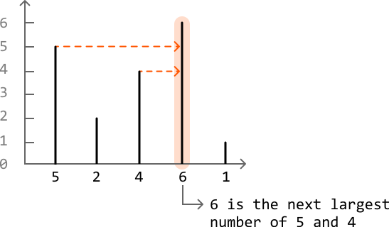
Bu nuqtai nazar o'zgarishi bilan massivni o'ngdan chapga qarab ko'rib chiqishimiz kerak.
Quyidagi misolni ko'rib chiqaylik:
![Image represents a bar chart illustrating a frequency distribution. The horizontal axis displays a sequence of numbers: [1, 1, 2, 3, 2, 3, 2, 4], representing data points. The vertical axis represents frequency, ranging from 0 to 4. Above each number on the horizontal axis, a vertical bar extends upwards to a height corresponding to its frequency of occurrence within the sequence. For instance, the number '1' appears twice, thus its bar reaches the height of '1' on the vertical axis; the number '2' appears three times, resulting in its bar reaching the height of '2'; the number '3' appears twice, reaching the height of '2'; and the number '4' appears once, reaching the height of '4'. The chart visually summarizes the frequency of each unique value in the given data set.](https://bytebytego.com/images/courses/coding-patterns/stacks/next-largest-number-to-the-right/image-07-02-2-Z7VU4XRS.svg?dpl=dpl_Gs7zfM6MUzjTBjcjps1LqXtb9QmD)
Eng o'ng indeksdan boshlaymiz, dastlab faqat 4 qiymatini bilamiz:
![Image represents a Cartesian coordinate system illustrating a data structure or algorithm, possibly related to candidate selection or a similar process. The horizontal axis depicts an array or list, labeled `[ ... 4 ]` at its ends, suggesting a sequence of elements where '4' is the last visible element, and ellipses (...) indicate unseen preceding elements. The vertical axis represents a numerical value or index, ranging from 0 to 4. A vertical line segment extends from the horizontal axis at the point labeled '4' to the top of the diagram, indicating a selection or operation focused on the element '4'. To the right, the text `candidates = []` shows an empty array or list named 'candidates', suggesting this structure might store selected elements. The text `res = []` similarly shows an empty array named 'res', likely representing the results or output of the process. The downward-pointing arrow above the vertical line suggests data flow or an operation being performed on the element '4'. The overall diagram likely visualizes a step in an algorithm where the element '4' is being processed or selected, with the 'candidates' and 'res' arrays potentially storing intermediate or final results.](https://bytebytego.com/images/courses/coding-patterns/stacks/next-largest-number-to-the-right/image-07-02-3-C2LMQVN6.svg?dpl=dpl_Gs7zfM6MUzjTBjcjps1LqXtb9QmD)
Hozircha 4 ni nomzod sifatida belgilashimiz mumkin.
![Image represents a Cartesian coordinate system illustrating a step in a coding pattern, possibly related to backtracking or a similar algorithm. The horizontal axis represents an index or iterator, with values implicitly ranging from an unspecified starting point to 4, indicated by the label `[... 4]`. The vertical axis represents a value or counter, ranging from 0 to 4. A vertical line segment extends from the horizontal axis at the point x=4, reaching a value of approximately 4 on the y-axis. To the right of the coordinate system, the text `candidates = [4]` indicates a list or array named `candidates` containing the single element 4. Below this, `res = [-1]` shows a list or array named `res` containing the single element -1, highlighted in a peach-colored box. The downward-pointing arrow above the vertical line suggests a process is occurring at index 4, potentially modifying the `res` array. The overall diagram likely visualizes a state within an iterative algorithm where the `candidates` list is being processed, and the `res` list is being updated.](https://bytebytego.com/images/courses/coding-patterns/stacks/next-largest-number-to-the-right/image-07-02-4-LKP2OZXK.svg?dpl=dpl_Gs7zfM6MUzjTBjcjps1LqXtb9QmD)
Keyingi 2 ni uchratamiz. 2 ning keyingi katta soni — eng so'nggi qo'shilgan nomzodlar ichidan 2 dan katta bo'lgan eng so'nggi nomzod.
4 ni 2 ning keyingi katta soni sifatida res ga yozing, so'ng 2 ni nomzodlar ro'yxatiga qo'shing.
![Image represents a Cartesian coordinate system illustrating a step in a coding algorithm, possibly related to backtracking or dynamic programming. The horizontal axis shows a range of values, with labeled points at 2 and 4, implying a discrete domain. The vertical axis represents a count or index, ranging from 0 to 4. Two vertical lines are drawn at x=2 and x=4, extending from the horizontal axis to y=2 and y=4 respectively. A dashed orange arrow points from the line at x=2 to the line at x=4, indicating a transition or step in the algorithm. Below the horizontal axis, `res = [ ... 4 -1]` is shown, suggesting a result array or list where '4' (highlighted in peach) is a current value and '-1' might represent a placeholder or a special value. To the right, `candidates = [4 2]` is displayed, indicating a list of candidate values used by the algorithm. The overall diagram visualizes a process where the algorithm moves from a state represented by the line at x=2 to a state represented by the line at x=4, updating the `res` array in the process, using values from the `candidates` list.](https://bytebytego.com/images/courses/coding-patterns/stacks/next-largest-number-to-the-right/image-07-02-5-HFSAGFWH.svg?dpl=dpl_Gs7zfM6MUzjTBjcjps1LqXtb9QmD)
Keyingi son 3. 3 ning kiritilishi bilan 2 endi nomzod bo'lmasligi kerak.
![Image represents a graphical illustration of a filtering process within a coding pattern, likely related to candidate selection or data pruning. A horizontal axis displays a sequence of numbers, including 2, 3, and 4, representing candidate values. Vertical lines of varying styles indicate the presence and status of these candidates. A solid black vertical line at '3' and '4' signifies that these candidates are initially present. A dashed red vertical line at '2' shows it as a candidate that will be removed. A downward-pointing grey arrow above the '3' suggests a filtering operation is being applied. To the right, the text 'remove all candidates ≤ 3:' in red describes the filtering criterion, while 'candidates = [4 2]' shows the initial candidates, and 'candidates = [4]' shows the candidates after filtering. Below, 'res = [4 -1]' likely represents the result of a subsequent operation on the remaining candidates. The vertical axis likely represents a frequency or some other metric, but its scale is not explicitly defined. The overall diagram visually demonstrates the removal of candidates based on a specified condition, resulting in a filtered set of candidates.](https://bytebytego.com/images/courses/coding-patterns/stacks/next-largest-number-to-the-right/image-07-02-6-UZ3BT3JX.svg?dpl=dpl_Gs7zfM6MUzjTBjcjps1LqXtb9QmD)
3 dan kichik yoki teng barcha nomzodlarni olib tashlaganimizdan so'ng, eng o'ng nomzod endi 4. 4 ni 3 ning keyingi katta soni sifatida yozamiz.
![Image represents a graphical depiction of a step in an algorithm, possibly related to candidate selection or a similar process. The core of the image is a Cartesian coordinate system with a horizontal x-axis and a vertical y-axis ranging from 0 to 4. Along the x-axis, a partially visible array `[ ... 3 2 4]` is shown, indicating a sequence of numbers. Two vertical lines, one black and one light gray, represent elements within this array. The black line is positioned at x=3 and extends vertically to y=3, while the light gray line is at x=2 and extends to y=1. A dashed orange arrow points horizontally from the top of the black line (at y=3) to a second black line positioned at x=4, extending vertically to y=4. Below the x-axis, the text `candidates = [4 3]` is displayed, suggesting these are the current candidates being considered. Additionally, `res = [ 4 4 -1]` is shown, likely representing the results or output of the algorithm so far, with the number 4 highlighted in a peach color. The downward-pointing gray arrow above the first black line indicates the current processing step. The overall diagram illustrates a transition or movement of data, possibly a value of 3, from one position in the array to another, updating the `candidates` and `res` arrays accordingly.](https://bytebytego.com/images/courses/coding-patterns/stacks/next-largest-number-to-the-right/image-07-02-7-2HFEIZWT.svg?dpl=dpl_Gs7zfM6MUzjTBjcjps1LqXtb9QmD)
Bu muhim tushuncha beradi:
Yangi son uchraganda, undan kichik yoki teng barcha nomzodlarni olib tashlash kerak.
Yana bir asosiy kuzatuv: nomzodlar ro'yxati doimo kamayib boruvchi tartibda saqlanadi.
![Image represents a bar graph combined with a line graph illustrating a coding pattern. The x-axis displays a sequence of numbers: [1, 1, 2, 3, 2, 3, 2, 4], representing an input array. Above each x-axis value, a vertical bar is drawn; the height of the bar corresponds to the values in a second array, `res = [2, 2, 3, 4, 3, 4, 4, -1]`, shown below the x-axis. The bars are black for positive values in `res` and light gray for the last value (-1). An orange line connects points representing a cumulative sum or another derived value from the `res` array. This line starts at (1,1) and increases with each subsequent point, indicating a trend. Separately, a rectangular box displays the array `candidates = [4, 3, 2, 1]`, which is labeled as 'decreasing,' indicating the array's elements are in descending order. An orange arrow points from the `candidates` array to the right, visually connecting it to the graph, suggesting that the `candidates` array is the input or a related data structure used to generate the graph's data.](https://bytebytego.com/images/courses/coding-patterns/stacks/next-largest-number-to-the-right/image-07-02-8-BMCWANAK.svg?dpl=dpl_Gs7zfM6MUzjTBjcjps1LqXtb9QmD)
Bu nomzodlar ro'yxatini saqlash uchun stack ideal ma'lumotlar tuzilmasi ekanligini ko'rsatadi.
Stackning tepasi har bir yangi son uchun o'ngdagi eng so'nggi nomzodni ifodalaydi.
- Stackning tepasidagi joriy qiymatdan kichik yoki teng barcha nomzodlarni olib tashlash.
- Stackning tepasi joriy qiymatning keyingi katta soni bo'ladi.
- Stackning tepasini joriy qiymat uchun javob sifatida yozing.
- Agar stack bo'sh bo'lsa, joriy qiymat uchun keyingi katta son yo'q. -1 ni yozing.
- Joriy qiymatni yangi nomzod sifatida stackga push qiling.
Amalga oshirish
from typing import List

def next_largest_number_to_the_right(nums: List[int]) -> List[int]:
    res = [0] * len(nums)
    stack = []
    # Find the next largest number of each element, starting with the rightmost
    # element.
    for i in range(len(nums) - 1, -1, -1):
        # Pop values from the top of the stack until the current value's next largest
        # number is at the top.
        while stack and stack[-1] <= nums[i]:
            stack.pop()
        # Record the current value's next largest number, which is at the top of the
        # stack. If the stack is empty, record -1.
        res[i] = stack[-1] if stack else -1
        stack.append(nums[i])
    return res
Murakkablik tahlili
Vaqt murakkabligi: next_largest_number_to_the_right ning vaqt murakkabligi O(n).
Xotira murakkabligi: Xotira murakkabligi O(n).
Ifodani Hisoblash
Ifodani Hisoblash
Butun sonlar, qavslar, qo'shish va ayirish amallarini o'z ichiga olgan matematik ifodani ifodalovchi matn berilgan. Ifodani hisoblang va natijani qaytaring.
Misol:
Input: s = '18-(7+(2-4))'
Output: 13
Fikrlash tarzi
Dastlab, turli elementlarni o'z ichiga olgan ifodalار bilan ishlash murakkab ko'rinishi mumkin. Keling, uni qismlarga ajrataylik.
Musbat va manfiy ishoralarni qayta ishlash Quyidagi ifodani ko'rib chiqing:

Bu ifodada ikkita ishora mavjud: plyus va minus. Ishora qiymatni o'zgartirish uchun ishlatilishi mumkin.

Ko'p raqamli sonlarni qayta ishlash Bu ifodadagi yana bir murakkablik — ba'zi sonlar bir necha raqamdan iborat.
"123" matni uchun bu jarayon quyidagi rasmlarda ko'rsatilgan:
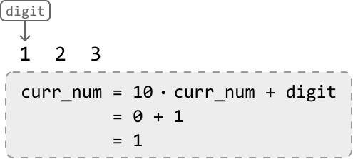
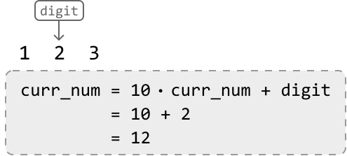
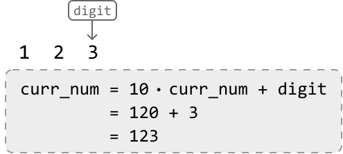
Raqam bo'lmagan belgi uchratilganda, sonni qurishni to'xtatamiz.
Qavssiz ifodani hisoblash Yuqoridagi ma'lumotlar asosida qavssiz ifodani hisoblaymiz.

'-' amaliga yetganimizda, birinchi son (28) tugagan. Shunday qilib:
- Joriy sonni (28) uning ishorasi bilan (1) ko'paytirish.
- Natijaga hosil bo'lgan ko'paytmani (28) qo'shish.
- Joriy amal minus ishorasi bo'lgani uchun ishorani -1 ga yangilash.
- Keyingi sonni qurishdan oldin curr_num ni 0 ga tiklash.

Ikkinchi amalga yetganimizda, joriy sonni (10) -1 ishorasi bilan ko'paytiriб natijaga qo'shamiz.

Nihoyat, matning oxiriga yetganimizda, oxirgi sonni (7) ishorasi bilan ko'paytirib natijaga qo'shamiz.

Qavsli ifodalarni hisoblash Endi oddiy ifodalarni hisoblashni bilganimizdan so'ng, qavsli ifodalarni ko'rib chiqaylik.
Bitta muammo — tashqi ifodani hisoblashdan oldin ichki ifodalar natijasini hisoblashimiz kerak.



Ushbu bobdagi qavslarni o'z ichiga olgan boshqa masala — To'g'ri Qavs Ifodasi — bu yerda ham foydali.
To'g'ri Qavs Ifodasi ga o'xshab, ochuvchi qavs '(' yangi ichki ifoda boshlanishini bildiradi.
Biz allaqachon qavssiz ifodalarni qanday hisoblashni bilamiz, shuning uchun faqat qavslar uchrashuvidagi harakatga e'tibor beramiz.
Birinchi ochuvchi qavsda yangi ichki ifoda boshlangani ma'lum. Ichki ifodani hisoblashdan oldin joriy holatni saqlaymiz.
Ochuvchi qavs uchraganda bajariluvchi qadamlar:
- stack.push(res): Joriy hisoblash natijasini stackga saqlash.
- stack.push(sign): Ichki ifoda ishorasini stackga saqlash.
- res = 0, sign = 1: Bu o'zgaruvchilarni tiklash, chunki yangi ifodani hisoblashni boshlaymiz.



Keyingi qavs ham ochuvchi qavs. Bu yangi ichki ifoda boshlanishini bildiradi.



Keyingi qavs yopuvchi qavs. Bu joriy ichki ifoda tugaganligini anglatadi.
- res *= stack.pop(): Joriy ichki ifodaga uning ishorasini tatbiq etish.
- res += stack.pop(): Tashqi ifoda natijasini joriy ichki ifoda natijasiga qo'shish.
Bu amallarni bajarganidan so'ng, res ning qiymati 5 bo'ladi.
Oxirgi yopuvchi qavsda ham xuddi shunday qadamlarni bajaramiz:
Nihoyat, res ning qiymati 13 bo'ladi, bu butun ifoda natijasini ifodalaydi.
Endi matning oxiriga yetganimizda, res ni qaytarishimiz mumkin.
Amalga oshirish
def evaluate_expression(s: str) -> int:
    stack = []
    curr_num, sign, res = 0, 1, 0
    for c in s:
        if c.isdigit():
            curr_num = curr_num * 10 + int(c)
        # If the current character is an operator, add 'curr_num' to the result
        # after multiplying it by its sign.
        elif c == '+' or c == '-':
            res += curr_num * sign
            # Update the sign and reset 'curr_num'.
            sign = -1 if c == '-' else 1
            curr_num = 0
        # If the current character is an opening parenthesis, a new nested expression
        # is starting.
        elif c == '(':
            # Save the current 'res' and 'sign' values by pushing them onto
            # the stack, then reset their values to start calculating the new nested
            # expression.
            stack.append(res)
            stack.append(sign)
            res, sign = 0, 1
        # If the current character is a closing parenthesis, a nested expression has
        # ended.
        elif c == ')':
            # Finalize the result of the current nested expression.
            res += sign * curr_num
            # Apply the sign of the current nested expression’s result before adding
            # this result to the result of the outer expression.
            res *= stack.pop()
            res += stack.pop()
            curr_num = 0
    # Finalize the result of the overall expression.
    return res + curr_num * sign
Murakkablik tahlili
Vaqt murakkabligi: evaluate_expression ning vaqt murakkabligi O(n) — matnning har bir belgisini bir marta ko'rib chiqamiz.
Xotira murakkabligi: Xotira murakkabligi O(n) — stack ichma-ich darajalariga mutanosib ravishda o'sishi mumkin.
Qo'shni Dublikatlarni Qayta-qayta Olib Tashlash
Qo'shni Dublikatlarni Qayta-qayta Olib Tashlash
Matn berilgan. Quyidagi amalni doimiy ravishda bajaring: qo'shni dublikat juftini matndan olib tashlang. Yana qo'shni dublikatlar qolmasa, natijani qaytaring.
-misol:

Input: s = 'aacabba'
Output: 'c'
-misol:

Input: s = 'aaa'
Output: 'a'
Fikrlash tarzi
Bu masaladagi asosiy qiyinchilik — hozircha qo'shni dublikat bo'lmagan belgilarni qanday boshqarish.
Matnni belgilar bo'yicha iterativ ravishda qurib, qo'shni dublikatlarni darhol olib tashlash strategiyasini sinab ko'rishimiz mumkin.
Boshqa qo'shni dublikat olib tashlanganidan so'ng yangi qo'shni dublikat hosil bo'lishi ham mumkin.
Quyidagi matnni ko'rib chiqaylik:

![Image represents a visual depiction of an algorithm, likely for string manipulation. The top section shows an input string 'a a c a b b a' preceded by a downward-pointing arrow originating from a square box labeled 'i,' suggesting an input indicator. This input string is then processed, resulting in a 'new string: a' displayed to the right. The bottom section mirrors the top, again showing the input string 'a a c a b b a' with the same input indicator 'i.' However, the resulting 'new string' is shown as 'a [a]' with a red line striking through the second 'a', indicating removal. A dashed-line box to the right of the bottom section labels this action as 'remove adjacent duplicate,' clarifying the algorithmic step performed. The overall diagram illustrates a process where adjacent duplicate characters are identified and removed from the input string.](https://bytebytego.com/images/courses/coding-patterns/stacks/repeated-removal-of-adjacent-duplicates/image-07-04-2-SUUW7EAK.svg?dpl=dpl_Gs7zfM6MUzjTBjcjps1LqXtb9QmD)
Ikkinchi 'a' ga yetganimizda, uni qo'shish qo'shni dublikatga olib kelishini sezamiz (ya'ni "aa" hosil bo'ladi).
Oxir-oqibat, qurayotgan matning natijasi faqat "c" bo'ladi.
Bu strategiya qanday ishlashini bilganimizdan so'ng, quyidagilarni amalga oshira oladigan ma'lumotlar tuzilmasi kerak:
- Uning bir uchiga harflar qo'shish.
- Xuddi shu uchidan harflarni olib tashlash.
Stack ma'lumotlar tuzilmasi bu ikkala amalni ham amalga oshirishga imkon beradi.
Belgilarni stackga push qilganimizda, stackning tepasi avvalgi/eng so'nggi belgini ifodalaydi.
- Joriy belgi stackning tepasidagi belgidan farqli bo'lsa, uni stackga push qiling.
- Joriy belgi stackning tepasidagi belgi bilan bir xil bo'lsa (ya'ni dublikat), stackning tepasini olib tashlang.
Barcha belgilar qayta ishlangandan so'ng, stackning mazmunini matn sifatida qaytarish kifoya.
Amalga oshirish
def repeated_removal_of_adjacent_duplicates(s: str) -> str:
    stack = []
    for c in s:
        # If the current character is the same as the top character on the stack,
        # a pair of adjacent duplicates has been formed. So, pop the top character
        # from the stack.
        if stack and c == stack[-1]:
            stack.pop()
        # Otherwise, push the current character onto the stack.
        else:
            stack.append(c)
    # Return the remaining characters as a string.
    return ''.join(stack)
Murakkablik tahlili
Vaqt murakkabligi: repeated_removal_of_adjacent_duplicates ning vaqt murakkabligi O(n) — har bir belgini bir marta ko'rib chiqamiz.
Xotira murakkabligi: Xotira murakkabligi O(n) — stack ko'pi bilan n ta belgini saqlaydi.
Stack Yordamida Queue Amalga Oshirish
Stack Yordamida Queue Amalga Oshirish
Stack ma'lumotlar tuzilmasidan foydalanib, queue ni amalga oshiring. Quyidagi funksiyalarni kiriting:
- enqueue(x: int) -> None: x ni queuening oxiriga qo'shadi.
- dequeue() -> int: queuening boshidagi elementni olib qaytaradi.
- peek() -> int: queuening boshidagi elementni qaytaradi.
Queue ni amalga oshirish uchun boshqa ma'lumotlar tuzilmalaridan foydalanmaslik kerak.
Misol
Input: [enqueue(1), enqueue(2), dequeue(), enqueue(3), peek()]
Output: [1, 2]
Cheklovlar:
- dequeue va peek amallari faqat bo'sh bo'lmagan queueda chaqiriladi.
Fikrlash tarzi
Queue birinchi kirgan birinchi chiqadi (FIFO) ma'lumotlar tuzilmasi, stack esa birinchi kirgan oxirida chiqadi (FILO) tamoyilida ishlaydi.
Bu ma'lumotlar tuzilmalarining asosiy farqi — elementlarni qanday chiqarishda. Queueda birinchi kirgani birinchi chiqadi, stackda esa aksincha.
Tushunib olganimizdan so'ng, masalaga kirishamiz. Bitta stack bilan queue ni amalga oshirish mumkinligini ko'raylik.
enqueue(1), enqueue(2), enqueue(3) buyruqlaridan keyin quyidagi stackni ko'ring:

dequeue amali bilan muammo yuzaga keladi — stackning tepasini olib tashlash so'nggi kiritilgan elementni qaytaradi, bu queue tamoyiliga zid.
Pastga yetish uchun stackning tepasidagi barcha qiymatlarni olib, vaqtinchalik saqlash kerak.
![Image represents a step-by-step visualization of a stack data structure's pop operation. Three diagrams show the stack's state at different points. Each diagram features a stack represented as a container with numbered elements (1, 2, 3) stacked vertically, with the top element indicated by 'top:'. A 'temp' array below each stack shows the elements popped so far. In the first diagram, a purple arrow labeled 'pop' shows the top element (3) being removed from the stack and added to the 'temp' array, which now contains [3]. The second diagram shows the next pop operation, with the top element (2) being removed and added to 'temp', resulting in [3, 2]. The third diagram shows the final pop operation, where the top element (1) is removed and the operation is labeled 'pop and return' in green, indicating the value is returned from the function. The 'temp' array remains [3, 2] as the stack is now empty.](https://bytebytego.com/images/courses/coding-patterns/stacks/implement-a-queue-using-stacks/image-07-05-3-AFS2TIBZ.svg?dpl=dpl_Gs7zfM6MUzjTBjcjps1LqXtb9QmD)
Pastdagi qiymatni (1) olib qaytarganimizdan so'ng, temp dagi qiymatlarni asosiy stackga qaytarib push qilish kerak.
![Image represents a step-by-step visualization of a stack data structure's behavior during a `push` operation. The image shows two stages. The leftmost stage depicts a stack labeled 'stack' containing the element '2', with 'top' indicating its position. A light-blue arrow labeled `push(2)` points to the stack, illustrating the addition of '2'. Below the stack, a dashed-line box displays a temporary variable `temp` holding the array `[3, 2]`. The next stage shows the stack after pushing the element '3' onto it. The element '3' is now at the top, with '2' below it. A light-blue arrow labeled `push(3)` shows the addition of '3'. The `temp` variable now holds `[3]`, reflecting the removal of '2' from the temporary storage. The overall image demonstrates how the `push` operation adds elements to the top of the stack and how a temporary variable might be used to manage data during this process.](https://bytebytego.com/images/courses/coding-patterns/stacks/implement-a-queue-using-stacks/image-07-05-4-EWG55UIF.svg?dpl=dpl_Gs7zfM6MUzjTBjcjps1LqXtb9QmD)
Agar temp kabi ma'lumotlar tuzilmasidan foydalansak, u stack bo'lishi kerak, chunki qiymatlarni teskari tartibda saqlashimiz kerak.
Bu yechim ishlasa ham, har bir dequeue amalida barcha elementlarni ko'chirishga to'g'ri keladi.

Asl yechimimizda temp dan asosiy stackga qiymatlarni qaytarib o'tkazardik. Ammo, agar yana dequeue chaqirilsa, ularni yana ko'chirishga to'g'ri keladi.
Shuning uchun, bu qiymatlarni asosiy stackga qaytarish o'rniga, tempda qoldirib, undan to'g'ridan-to'g'ri qaytarish mumkin.
Yuqoridagi mantiqda ikkita stack bor, har biri o'z maqsadiga xizmat qiladi:
- Har bir enqueue chaqiruvida qiymatlarni push qiladigan stack (enqueue_stack).
- Har bir dequeue chaqiruvida qiymatlarni pop qiladigan stack (dequeue_stack).
E'tibor bering: dequeue stack doimo qiymatlar bilan to'ldirilmaydi. Faqat bo'sh bo'lganda enqueue stack dan to'ldiriladi.
Ikkita enqueue chaqiruvi bilan boshlaymiz va har bir sonni enqueue stackga push qilamiz.
Keling, dequeue chaqiruvini qayta ishlaylik. Birinchi qadam — enqueue stackdagi har bir elementni dequeue stackga ko'chirish.
Keyin dequeue stackning tepasidagi qiymatni qaytaramiz:
Yana bitta qiymatni enqueue qilamiz:
dequeue ni yana chaqirsak, dequeue stackning tepasidagi qiymatni qaytaramiz:
Endi dequeue chaqirilganda dequeue stack bo'sh bo'lsa? Enqueue stackdagi barcha elementlarni ko'chirib to'ldirish kerak.
peek funksiyasi uchun dequeue funksiyasi bilan bir xil mantiq qo'llaniladi, lekin element olinmaydi, faqat qaytariladi.
Amalga oshirish
Yuqorida aytib o'tilganidek, dequeue va peek funksiyalari deyarli bir xil mantiqqa ega, yagona farq dequeue element olib qaytaradi, peek esa faqat qaytaradi.
class Queue:
    def __init__(self):
        self.enqueue_stack = []
        self.dequeue_stack = []

    def enqueue(self, x: int) -> None:
        self.enqueue_stack.append(x)

    def transfer_enqueue_to_dequeue(self) -> None:
        # If the dequeue stack is empty, push all elements from the enqueue stack
        # onto the dequeue stack. This ensures the top of the dequeue stack
        # contains the most recent value.
        if not self.dequeue_stack:
            while self.enqueue_stack:
                self.dequeue_stack.append(self.enqueue_stack.pop())

    def dequeue(self) -> int:
        self.transfer_enqueue_to_dequeue()
        # Pop and return the value at the top of the dequeue stack.
        return self.dequeue_stack.pop() if self.dequeue_stack else None

    def peek(self) -> int:
        self.transfer_enqueue_to_dequeue()
        return self.dequeue_stack[-1] if self.dequeue_stack else None
Murakkablik tahlili
Vaqt murakkabligi:
- enqueue O(1) — enqueue stackga bitta element qo'shamiz.
- dequeue amortizatsiya qilingan O(1). Eng yomon holatda, enqueue stackdagi barcha elementlar dequeue stackga ko'chiriladi. Ammo har bir element ko'pi bilan bir marta ko'chiriladi, shuning uchun amortizatsiya qilingan narxi O(1).
- peek amortizatsiya qilingan O(1) — dequeue bilan bir xil sabab.
Xotira murakkabligi: Xotira murakkabligi O(n) — ikkala stack birga n ta elementni saqlaydi.
Siljuvchi Oyna Maksimumlari
Siljuvchi Oyna Maksimumlari
k o'lchamli siljuvchi oyna butun sonlar massivi bo'ylab chapdan o'ngga siljiydi. Har bir oyna pozitsiyasidagi maksimal qiymatlardan iborat massiv yarating.
Misol:
![Image represents a step-by-step illustration of finding the maximum value within an array of integers. Four rows depict the array `[3, 2, 4, 1, 2, 1, 1]`. In each row, a light-blue rectangular highlight progressively moves across the array, indicating the current element being considered as the potential maximum. To the right of each array, 'max = ' is followed by the maximum value found so far during that step. The first three rows show the highlight moving from the leftmost element (3) to the element 4, correctly identifying 4 as the maximum. The final row shows the highlight moving to the last element (1) after 4 has already been identified as the maximum, resulting in a final maximum value of 4. The image visually demonstrates a linear scan algorithm for finding the maximum element in an array.](https://bytebytego.com/images/courses/coding-patterns/stacks/maximums-of-sliding-window/maximums-of-sliding-window-ZTLN5HJK.svg?dpl=dpl_Gs7zfM6MUzjTBjcjps1LqXtb9QmD)
Input: nums = [3, 2, 4, 1, 2, 1, 1], k = 4
Output: [4, 4, 4, 2]
Fikrlash tarzi
Qo'pol kuch yondashuvi har bir oyna ichidagi har bir elementni ko'rib chiqishni o'z ichiga oladi. Bu O(n*k) vaqt oladi.
Asosiy muammo — oyna sirpanganda, biz allaqachon ko'rgan elementlarni qayta tekshirib chiqamiz.
![Image represents two nearly identical arrays of integers, each enclosed in square brackets. The top array is `[3, 2, 4, 1, 2, 1, 1]` and the bottom array is `[3, 2, 4, 1, 2, 1, 1]`. A light-blue rectangular box highlights the sub-array `[2, 4, 1]` in both arrays, indicating that these elements have the same values in both arrays. The text 'same values' is positioned within the central area of the box, explicitly labeling the highlighted section. The arrays are horizontally aligned, with the highlighted sections overlapping vertically. No URLs or parameters are present.](https://bytebytego.com/images/courses/coding-patterns/stacks/maximums-of-sliding-window/image-07-06-1-ZWBRMHOR.svg?dpl=dpl_Gs7zfM6MUzjTBjcjps1LqXtb9QmD)
Yanada samarali yechim — ixtiyoriy oynaning maksimumini tezda aniqlash uchun ko'rilgan qiymatlarni kuzatib borishni o'z ichiga oladi.
Quyidagi massivdagi k=4 o'lchamli oynani ko'rib chiqaylik. left va right ko'rsatkichlar oynani belgilaydi.
![Image represents a visual depiction of data partitioning or splitting. Two rectangular boxes labeled 'left' and 'right' are positioned above a horizontal array of numbers: [3, 2, 4, 1, 2, 1, 1]. Arrows descend from 'left' and 'right' pointing to the number array. The numbers 3, 2, 4, and 1 are highlighted with a light blue background, indicating that this section of the array is associated with the 'left' box. The remaining numbers (2, 1, 1) are not highlighted and are implicitly associated with the 'right' box. The diagram illustrates how a data set (the array of numbers) is divided into two subsets, 'left' and 'right,' based on some unspecified criteria.](https://bytebytego.com/images/courses/coding-patterns/stacks/maximums-of-sliding-window/image-07-06-2-U6W6S5Z2.svg?dpl=dpl_Gs7zfM6MUzjTBjcjps1LqXtb9QmD)
Keyingi oyna uchun nomzodlarni aniqlash uchun har bir sonni alohida ko'rib chiqaylik.
3: Son 3 joriy oyna uchun nomzod, ammo keyingi oynaga o'tganimizda, o'ng tomonidan chiqib ketgani uchun uni e'tiborsiz qoldirishimiz mumkin.
2: Son 2 keyingi oynaning maksimumi bo'la oladimi? Yo'q. Chunki o'ng tomonida 4 bor, u 2 dan katta va oynada uzoqroq qoladi.
4: Bu joriy oynaning maksimal qiymati va ba'zi kelgusi oynalarda ham bo'ladi. Uni nomzod sifatida saqlaymiz.
1: 1 kelgusi oynaning maksimumi bo'la oladimi? Ha. 4 hozir katta bo'lsa-da, oyna udan chiqib ketgandan keyin 1 maksimum bo'lishi mumkin.
Yuqoridagi tahlil asosida oyna yangi element uchrashuvidagi strategiya:
- Kichikroq yoki teng nomzodlarni olib tashlash: Yangi nomzoddan kichik yoki unga teng bo'lgan mavjud nomzodlar olib tashlanadi.
- Yangi nomzod qo'shish: Kichikroq nomzodlar tashlangandan so'ng, yangi qiymat nomzod sifatida qo'shiladi.
- Eskirgan nomzodlarni olib tashlash: Oyna biror qiymatdan o'tib ketganda, u qiymat nomzodlar ro'yxatidan chiqarilishi kerak.
Bu strategiya oyna bir indeks oldinga siljiganda nomzodlar ro'yxatiga qanday tatbiq etilishini ko'ring:
![Image represents a sliding window algorithm visualization. The initial state shows a numerical array `nums = [2 5 4 3 2 1 3]` where a light-blue rectangle highlights a window encompassing the elements [2 5 4 3 2 1]. A thick grey arrow labeled 'slide window' indicates a rightward shift of this window. The resulting state shows a new window [2 5 4 3 2 1 3] where the element '2' is no longer in the window (indicated by text 'no longer in window' and a downward arrow pointing to the new window), and a new element '3' has entered the window (indicated by text 'new candidate' and a downward arrow pointing to the '3' within the new window). The '3' in the new window is highlighted with a light grey circle to emphasize its addition. The overall diagram illustrates a single iteration of a sliding window technique, showing how the window moves across the array, adding and removing elements.](https://bytebytego.com/images/courses/coding-patterns/stacks/maximums-of-sliding-window/image-07-06-3-CVTTGXKJ.svg?dpl=dpl_Gs7zfM6MUzjTBjcjps1LqXtb9QmD)
![Image represents a step-by-step process demonstrating a coding pattern, likely related to candidate selection or filtering. It begins with an initial list of candidates: `[5 4 3 2 1]`. Step 1, labeled 'remove values ≤ new candidate (3)', shows the removal of values 3, 2, and 1 from the list, resulting in `[5 4]`. A red line visually connects the removed elements. Step 2, 'add the new candidate', inserts the value '3' (in orange) into the list, producing `[5 4 3]`. Finally, step 3, 'remove outdated values', removes the value 5 (indicated by a red line), leaving the final list as `[4 3]`. The process illustrates a sequence of operations involving removing elements based on a condition, adding a new element, and then potentially removing further elements based on another criteria, possibly to maintain a specific list size or order.](https://bytebytego.com/images/courses/coding-patterns/stacks/maximums-of-sliding-window/image-07-06-4-222NXXJE.svg?dpl=dpl_Gs7zfM6MUzjTBjcjps1LqXtb9QmD)
Muhim kuzatuv: nomzod qiymatlar doimo kamayib boruvchi tartibda saqlanadi. Chunki yangi nomzoddan kichik yoki teng bo'lgan qiymatlar olib tashlanadi.
Shuning uchun oyna uchun maksimal qiymat doimo nomzodlar ro'yxatining birinchi qiymati bo'ladi.
Shunday qilib, nomzodlarni saqlash uchun monoton kamayuvchi tartibdagi qiymatlarni saqlash hamda ikkala uchidan qo'shish va olib tashlash imkonini beruvchi ma'lumotlar tuzilmasi kerak.
Deque Odatda stack monoton kamayuvchi tartibdagi qiymatlarni saqlash uchun ishlatiladi. Ammo stackdan faqat bir uchidan olib tashlash mumkin.
Ikkala uchidan ham qo'shish va olib tashlash imkonini beradigan ma'lumotlar tuzilmasi mavjudmi? Ha — double-ended queue yoki deque.
Nomiga qaramay, deque ni ikkala uchli stack sifatida tasavvur qilish osonroq:
![Image represents a comparison of stack and deque data structures. The left side depicts a stack, labeled 'stack:', showing a linear array represented by `[• • • • • •]`. A cyan-colored arrow labeled 'push' indicates that new elements are added to the right end. Conversely, a purple arrow labeled 'pop' shows that elements are removed from the right end (LIFO - Last In, First Out). The right side illustrates a deque, labeled 'deque:', also represented by a linear array `[• • • • • •]`. However, unlike the stack, the deque has two cyan arrows indicating 'push to left' and 'push to right,' signifying that elements can be added to either end. Similarly, two purple arrows, 'pop from left' and 'pop from right,' demonstrate that elements can be removed from both the left and right ends (FIFO - First In, First Out from one end, and LIFO from the other). The overall image visually contrasts the unidirectional nature of stack operations with the bidirectional capabilities of deque operations.](https://bytebytego.com/images/courses/coding-patterns/stacks/maximums-of-sliding-window/image-07-06-5-U6LM7UCU.svg?dpl=dpl_Gs7zfM6MUzjTBjcjps1LqXtb9QmD)
Endi ma'lumotlar tuzilmamiz bor, keling uni quyidagi misol ustida qanday ishlatishni ko'raylik. Deque indekslarni saqlaydi, qiymatlarni emas.
![Image represents a depiction of a queue data structure, showing its initial state and an empty dequeued queue. A numerical array `[3, 2, 4, 1, 2, 1, 1]` is presented, representing the elements of the queue. Beneath each element, a numerical index (0 to 6) indicates its position within the queue. A comma separates the queue array from the representation of the dequeued queue, denoted as `dq = []`, which is an empty array, signifying that no elements have been removed from the original queue yet. The arrangement visually displays the queue's contents and its index-based organization, with the `dq` variable clearly showing the absence of dequeued elements.](https://bytebytego.com/images/courses/coding-patterns/stacks/maximums-of-sliding-window/image-07-06-6-MEB3MP6S.svg?dpl=dpl_Gs7zfM6MUzjTBjcjps1LqXtb9QmD)
Oyna k uzunligiga yetguncha kengaytiring. Har bir uchrashadigan nomzod uchun monoton kamayuvchi tartibni ta'minlashimiz kerak.
![Image represents a visual explanation of a coding pattern, likely involving a deque (double-ended queue) data structure. At the top, two rectangular boxes labeled 'left' and 'right' point downwards with arrows towards an array `[3, 2, 4, 1, 2, 1, 1]`. The number 3 at index 0 is highlighted in light blue, indicating a focus on this element. To the right, two separate, light-grey, dashed-bordered boxes describe operations: the top box states '1) pop candidates ≤ 3', suggesting elements from the array are popped (removed) until a condition (candidates ≤ 3) is met. The bottom box describes '2) push 3 with its index', indicating that the value 3 (and potentially its index 0) is added to another data structure. Finally, an equation `dq = [(3, 0)]` is shown, where `dq` likely represents the deque, and `[(3, 0)]` shows the deque's content after the operations, containing the value 3 paired with its original index 0. The `val` and `index` labels below clarify the tuple's structure within the deque. The entire diagram illustrates a step-by-step process of manipulating an array and updating a deque based on a specific condition.](https://bytebytego.com/images/courses/coding-patterns/stacks/maximums-of-sliding-window/image-07-06-7-B2NZMCHS.svg?dpl=dpl_Gs7zfM6MUzjTBjcjps1LqXtb9QmD)
![Image represents a visual explanation of a coding pattern, likely involving a deque (double-ended queue) data structure. The top-left shows two labeled boxes, 'left' and 'right,' pointing downwards to an array `[3, 2, 4, 1, 2, 1, 1]`. The numbers 0 through 6 underneath the array represent their indices. The numbers 3 and 2 are highlighted in light blue, indicating they are initial candidates. Two rectangular boxes on the right describe a two-step process: 1) 'pop candidates ≤ 2,' suggesting elements with values less than or equal to 2 are removed from the array; and 2) 'push 2 with its index,' indicating that the value 2 and its index (1) are added to a new data structure. The result of this process is shown as `dq = [(3, 0), (2, 1)]`, where `dq` represents the deque, and each tuple contains a value and its original index from the input array. An arrow labeled 'decreasing values' points to the right, indicating that the deque is ordered by decreasing values.](https://bytebytego.com/images/courses/coding-patterns/stacks/maximums-of-sliding-window/image-07-06-8-R4B66OH2.svg?dpl=dpl_Gs7zfM6MUzjTBjcjps1LqXtb9QmD)
4 ga yetganimizda, uni darhol dequega qo'sha olmaymiz, chunki bu monoton kamayuvchi tartibni buzadi.
![Image represents a visual explanation of a coding pattern, likely involving a deque (dq) data structure and a sorting or searching algorithm. The top left shows an array `[3, 2, 4, 1, 2, 1, 1]` with indices 0-6. Arrows labeled 'left' and 'right' point to the elements 3 and 4 respectively, suggesting these are initial boundary points. A dashed box to the right describes a 'pop' operation (step 1) where elements are removed if their value is less than or equal to 4. To the right of this, the deque `dq` is initialized as `[(3, 0), (2, 1)]`, representing value-index pairs. Below, another dashed box describes a 'push' operation (step 2) where the element 4 (at index 2) is added to the deque. The subsequent `dq` becomes `[(4, 2)]`. Red arrows and inequalities (4 > 2, 4 > 3) illustrate comparisons between the current element being considered (4) and elements already in the deque, indicating a process of maintaining a sorted or prioritized subset within the deque. The labels 'val' and 'index' clearly denote the components of each pair within the deque.](https://bytebytego.com/images/courses/coding-patterns/stacks/maximums-of-sliding-window/image-07-06-9-UQZYURAK.svg?dpl=dpl_Gs7zfM6MUzjTBjcjps1LqXtb9QmD)
Oynaning keyingi kengayishi kutilgan k o'lchamni o'rnatadi:
![Image represents a visualization of a coding pattern, likely involving a deque (double-ended queue) data structure. The top-left shows an array `[3, 2, 4, 1, 2, 1, 1]` with a pointer `k` positioned at index 2, indicating a potential split point. Above the array, boxes labeled 'left' and 'right' suggest the array is being processed from both ends. A light-blue highlight spans the array from index 0 to index 3, possibly representing a processed section. The right side displays two labeled boxes describing steps in an algorithm: 1) 'pop candidates ≤ 1' implying elements less than or equal to 1 are removed, and 2) 'push 1 with its index' suggesting that the value 1 and its index are added to a data structure. The result of this algorithm is shown as `dq = [(4, 2), (1, 3)]`, a deque containing pairs where the first element is the value and the second is its original index, arranged in decreasing order of values, as indicated by the arrow labeled 'decreasing values'. The `dq` represents the output after processing the array according to the described steps.](https://bytebytego.com/images/courses/coding-patterns/stacks/maximums-of-sliding-window/image-07-06-10-N5UM4WCH.svg?dpl=dpl_Gs7zfM6MUzjTBjcjps1LqXtb9QmD)
Oyna k uzunligiga yetgandan so'ng, har bir oynaning maksimal qiymatini qayd etish vaqti keldi. Yuqorida aytib o'tilganidek, deque ning boshi maksimal qiymatni ifodalaydi.
Oyna k o'lchamga yetgandan so'ng, yondashuvimiz oynani kengaytirishdan sirpantishga o'tadi.
![Image represents a visualization of a coding pattern, likely involving a deque (dq) data structure and a sliding window technique. The top-left shows an array `[3, 2, 4, 1, 2, 1]` with indices 0-6. Arrows labeled 'left' and 'right' point to elements 2 and 2 respectively, indicating a window's boundaries. Three numbered, dashed-bordered boxes describe the algorithm's steps: 1) 'pop candidates ≤ 2' which, alongside the right-hand side, shows an initial deque `dq = [(4, 2), (1, 3)]` where each pair represents (value, index) and the element (1,3) is removed because its value is less than or equal to 2; 2) 'push 2 with its index' resulting in `dq = [(4, 2), (2, 4)]`; and 3) 'remove outdated candidates,' which is not explicitly shown in the deque but implies further processing. The right-hand side illustrates the deque's evolution, with a red arrow highlighting the removal of (1,3) and the final deque showing pairs ordered by decreasing values, indicating the algorithm maintains a sorted deque of candidates within the sliding window.](https://bytebytego.com/images/courses/coding-patterns/stacks/maximums-of-sliding-window/image-07-06-11-KHZ44AFZ.svg?dpl=dpl_Gs7zfM6MUzjTBjcjps1LqXtb9QmD)
Bu uch amaldan keyin oynaning maksimal qiymati 4 ekanligi aniqlanadi.
![Image represents a step-by-step illustration of a coding pattern, likely involving a deque (double-ended queue) data structure. The top shows an array `[3, 2, 4, 1, 2, 1]` with indices 0-6. Arrows labeled 'left' and 'right' point to the element '4' and '1' respectively, indicating a focus on a sub-array. Below, three numbered steps describe operations on a deque (`dq`). Step 1) 'pop candidates ≤ 1' suggests removing elements from the deque with values less than or equal to 1. Step 2) 'push 1 with its index' indicates adding the element '1' along with its index (in this case, index 5) to the deque. The result of step 2 is shown as `dq = [(4, 2), (2, 4), (1, 5)]`, where each tuple represents (value, index) pairs, ordered by decreasing values as indicated by the arrow. Finally, step 3) 'remove outdated candidates' implies removing elements from the deque that are no longer relevant based on the algorithm's logic. The entire diagram visualizes the process of maintaining a deque of candidates, ordered by decreasing values, within a specific algorithm.](https://bytebytego.com/images/courses/coding-patterns/stacks/maximums-of-sliding-window/image-07-06-12-CI6XFS4I.svg?dpl=dpl_Gs7zfM6MUzjTBjcjps1LqXtb9QmD)
Bu uch amaldan keyin oynaning maksimal qiymati ham 4 — u hali deque da.
![Image represents a step-by-step illustration of a coding pattern, likely involving a deque (dq) data structure and a sliding window or similar algorithm. The top shows an array `[3, 2, 4, 1, 2, 1, 1]` with indices 0-6, and arrows pointing from labels 'left' and 'right' to the array's element at index 3 and 6 respectively. Below, three numbered steps are shown, each accompanied by a description and the evolution of the deque `dq`. Step 1, 'pop candidates ≤ 1', shows `dq` initially containing pairs (value, index) representing elements from the array: `[(4, 2), (2, 4), (1, 5)]`. A red arrow indicates the removal of `(1, 5)` because its value (1) meets the condition. Step 2, 'push 1 with its index', adds `(1, 6)` to `dq`, resulting in `[(4, 2), (2, 4), (1, 6)]`. The arrow indicates the deque is ordered by decreasing values. Step 3, 'remove outdated candidates', removes `(4,2)` from `dq` because its index (2) is less than the current `left` pointer (indicated by a red arrow pointing to `(4,2)` and the inequality `2 < left`). The final `dq` is `[(4, 2), (2, 4), (1, 6)]` after this step. The overall process demonstrates how the deque maintains a subset of the array's elements based on value and index, dynamically adapting to the movement of the `left` and `right` pointers.](https://bytebytego.com/images/courses/coding-patterns/stacks/maximums-of-sliding-window/image-07-06-13-WXWFI2UB.svg?dpl=dpl_Gs7zfM6MUzjTBjcjps1LqXtb9QmD)
Bu oynaning maksimal qiymatini qayd etishdan oldin, 4 ning oynadan chiqib ketgani uchun dequeden olib tashlashimizni ta'minladik.
Amalga oshirish
from typing import List
from collections import deque

def maximums_of_sliding_window(nums: List[int], k: int) -> List[int]:
    res = []
    dq = deque()
    left = right = 0
    while right < len(nums):
        # 1) Ensure the values of the deque maintain a monotonic decreasing order
        # by removing candidates <= the current candidate.
        while dq and dq[-1][0] <= nums[right]:
            dq.pop()
        # 2) Add the current candidate.
        dq.append((nums[right], right))
        # If the window is of length 'k', record the maximum of the window.
        if right - left + 1 == k:
            # 3) Remove values whose indexes occur outside the window.
            if dq and dq[0][1] < left:
                dq.popleft()
            # The maximum value of this window is the leftmost value in the
            # deque.
            res.append(dq[0][0])
            # Slide the window by advancing both 'left' and 'right'. The right
            # pointer always gets advanced so we just need to advance 'left'
            left += 1
        right += 1
    return res
Murakkablik tahlili
Vaqt murakkabligi: maximums_of_sliding_window ning vaqt murakkabligi O(n) — massiv bo'ylab bir marta o'tamiz.
Xotira murakkabligi: Xotira murakkabligi O(k) — deque ko'pi bilan k ta elementni saqlaydi.
Intervyu maslahati
Maslahat: Agar masala uchun qaysi ma'lumotlar tuzilmasidan foydalanishni bilmasangiz, avval qanday xususiyatlar kerakligini aniqlang va keyin shu xususiyatlarga mos keladigan ma'lumotlar tuzilmasini toping.
Heap-lar
Heap-larga Kirish
Heap-larga Kirish
Intuitsiya
Heap — elementlarni ustuvorlik asosida tartiblaydigan ma'lumotlar strukturasi bo'lib, eng yuqori ustuvorlikdagi element doimo heap tepasida bo'lishini ta'minlaydi. Bu istalgan vaqtda eng yuqori ustuvorlikdagi elementga samarali kirish imkonini beradi. Heap-larning ikkita asosiy turi mavjud:
- Min-heap: eng kichik elementni ustuvor qilib, uni heap tepasida saqlaydi.
- Max-heap: eng katta elementni ustuvor qilib, uni heap tepasida saqlaydi.
Samarali ustuvorlashtirish heap-larning tuzilishi tufayli mumkin. Heap aslida ikkilik daraxt hisoblanadi. Masalan, min-heap holatida har bir tugunning qiymati o'z farzandlarining qiymatidan kichik yoki teng bo'ladi. Bu daraxtning ildizi (heap tepasi) doimo eng kichik element ekanligini kafolatlaydi:
Umumiy heap operatsiyalarining vaqt murakkabligi:
Ushbu bob heap-larning amaliy qo'llanishlarini muhokama qiladi. Heap qanday ishlashini chuqurroq tushunish uchun uning ichki amalga oshirilishi va turli operatsiyalar davomida ikkilik daraxt tuzilishi qanday saqlanishi bilan tanishishni tavsiya etamiz [2].
Ustuvorlik navbati: Ustuvorlik navbati — min-heap yoki max-heap tuzilishiga amal qiluvchi, ammo elementlarni ustuvorlash usulini moslashtirish imkonini beruvchi maxsus heap turi.
Hayotiy Misol
Operatsion tizimlarda vazifalarni boshqarish: Operatsion tizimlar ko'pincha vazifalar bajarilishini boshqarish uchun ustuvorlik navbatidan foydalanadi, va heap bu ustuvorlik navbatini samarali amalga oshirish uchun keng qo'llaniladi.
Masalan, kompyuterda bir nechta jarayon ishlayotganda, har bir jarayonga ustuvorlik darajasi belgilanishi mumkin. Operatsion tizim jarayonlarni shunday rejalashtirishi kerakki, yuqori ustuvorlikdagi vazifalar pastroq ustuvorlikdagilardan oldin bajarilsin.
Bob Rejasi
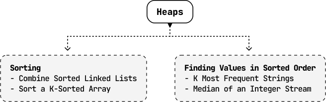
K Ta Eng Ko'p Uchraydigan Satrlar
K Ta Eng Ko'p Uchraydigan Satrlar
Massivdagi k ta eng ko'p uchraydigan satrlarni toping va ularni chastota bo'yicha kamayish tartibida qaytaring. Ikki satrning chastotasi bir xil bo'lsa, ularni leksikografik tartibda saralang.
Misol:
Input: strs = ['go', 'coding', 'byte', 'byte', 'go', 'interview', 'go'], k = 2
Output: ['go', 'byte']
Tushuntirish: "go" va "byte" satrlari eng ko'p uchraydi, mos ravishda 3 va 2 marta.
Cheklovlar:
- k ≤ n, bu yerda n massiv uzunligini bildiradi.
Intuitsiya - Max-Heap
Bu masalaning ikkita asosiy qiyinligi:
- K ta eng ko'p uchraydigan satrlarni aniqlash.
- Bu satrlarni avval chastota, keyin leksikografik tartibda saralash.
Avval har bir satrning chastotasini kuzatib borishimiz kerak. Buning uchun hash map ishlatishimiz mumkin: kalitlar satrlarni, qiymatlar esa chastotalarni ifodalaydi.
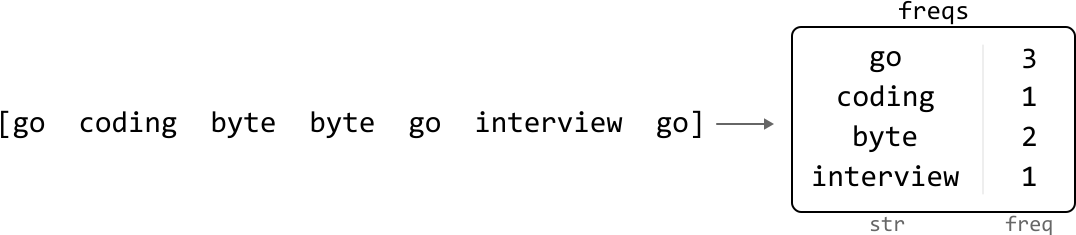
Eng oddiy yondashuv — hash map'dan satrlarni o'z ichiga olgan massiv olish va uni chastota bo'yicha kamayish tartibida saralash. K ta eng ko'p uchraydigan satrlar bu massivning dastlabki k ta elementi bo'ladi.
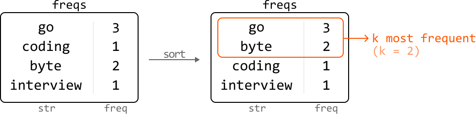
Bu yechimning asosiy samarasizligi shundaki, faqat k ta eng ko'p uchraydigan satrni saralash kerak bo'lsa-da, barcha n ta satr sarаlanadi.
Foydali kuzatuv: agar eng ko'p uchraydigan satrni olib tashlasak, qolganlar orasidagi eng ko'p uchraydigan satr ikkinchi o'rindagi bo'ladi. Eng ko'p uchraydigan satrni k marta ketma-ket aniqlab olib tashlash orqali javobni samarali topamiz.
Bu g'oyani amalga oshirish uchun istalgan vaqtda eng ko'p uchraydigan satrga samarali kirish imkonini beruvchi ma'lumotlar strukturasi kerak. Buning uchun max-heap juda qulay.
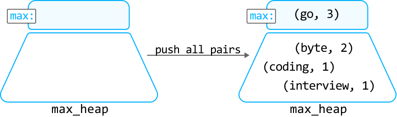
Heap-ni to'ldirish uchun barcha n ta satrni bittadan qo'shish mumkin, bu O(nlog(n)) vaqt oladi. Buning o'rniga, barcha satr-chastota juftliklarini o'z ichiga olgan massivda heapify operatsiyasini bajarib, max-heap'ni O(n) vaqtda yaratishimiz mumkin.
K ta eng ko'p uchraydigan satrlarni yig'ish uchun heap tepasidan k marta element olib, mos satrlarni res natija massiviga saqlang:
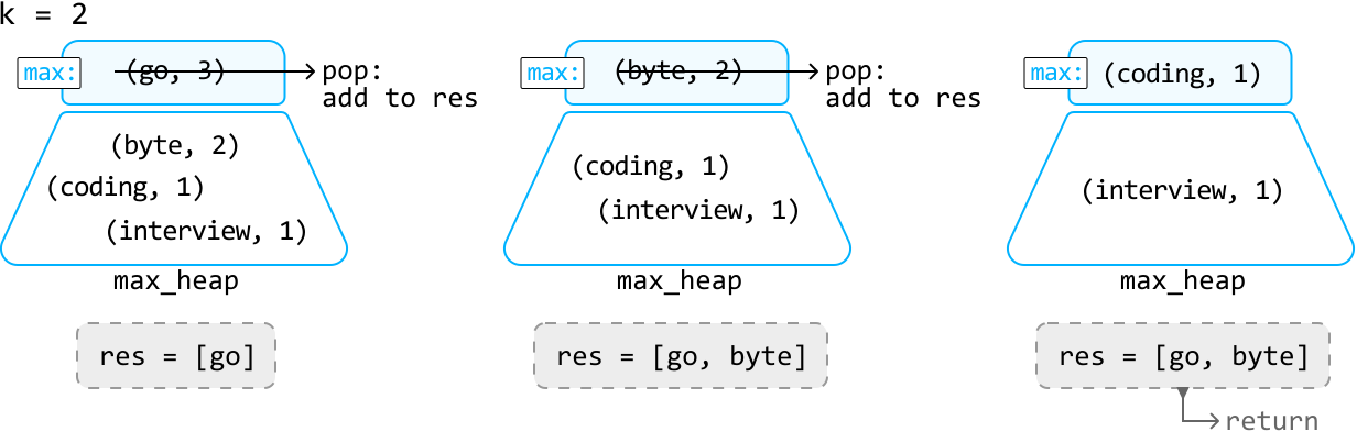
Endi, chastotasi bir xil bo'lgan ikkita satrda leksikografik jihatdan birinchi keladigani heap'da yuqori ustuvorlikka ega bo'lishini ta'minlashimiz kerak. Buning uchun heap uchun maxsus taqqoslagich (comparator) belgilashimiz mumkin.
Amalga Oshirish - Max-Heap
Satr-chastota juftliklari uchun Pair klassi yaratamiz va maxsus taqqoslagich yordamida ustuvorlikni moslashtirish imkonini beramiz.
from typing import List
from collections import Counter
import heapq

class Pair:
   def __init__(self, str, freq):
       self.str = str
       self.freq = freq

   def __lt__(self, other):
       if self.freq == other.freq:
           return self.str < other.str
       return self.freq > other.freq

def k_most_frequent_strings_max_heap(strs: List[str], k: int) -> List[str]:
   freqs = Counter(strs)
   max_heap = [Pair(str, freq) for str, freq in freqs.items()]
   heapq.heapify(max_heap)
   return [heapq.heappop(max_heap).str for _ in range(k)]
Murakkablik Tahlili
Vaqt murakkabligi: O(n + k log(n)). Xotira murakkabligi: O(n).
Intuitsiya - Min-Heap
Davomiy savol sifatida suhbatdosh heap tomonidan ishlatiladigan xotirani kamaytirish uchun yechimingizni o'zgartirishni so'rashi mumkin.
Muhim kuzatuv: heap hajmi k dan oshib ketganda, eng kam chastotali satrlarni heap hajmi yana k ga qadar kamayguncha olib tashlashimiz mumkin. Buni qila olamiz, chunki olib tashlangan satrlar k ta eng ko'p uchraydigan satrlar orasida bo'lmaydi.
Ammo bu strategiyani max-heap bilan amalga oshirib bo'lmaydi, chunki eng kam chastotali satrga kirish imkonimiz bo'lmaydi. Buning o'rniga min-heap ishlatishimiz kerak.
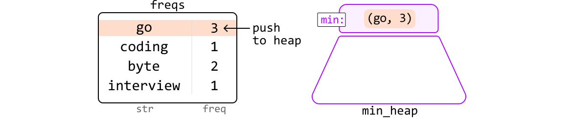
from typing import List
from collections import Counter
import heapq

class Pair:
    def __init__(self, str, freq):
        self.str = str
        self.freq = freq
    def __lt__(self, other):
        if self.freq == other.freq:
            return self.str > other.str
        return self.freq < other.freq

def k_most_frequent_strings_min_heap(strs: List[str], k: int) -> List[str]:
    freqs = Counter(strs)
    min_heap = []
    for str, freq in freqs.items():
        heapq.heappush(min_heap, Pair(str, freq))
        if len(min_heap) > k:
            heapq.heappop(min_heap)
    return [heapq.heappop(min_heap).str for _ in range(k)][::-1]
Murakkablik Tahlili
Vaqt murakkabligi: O(n log(k)). Xotira murakkabligi: hash map uchun O(n), heap uchun O(k).
Saralangan Bog'liq Ro'yxatlarni Birlashtirish
Saralangan Bog'liq Ro'yxatlarni Birlashtirish
Ko'tarilish tartibida saralangan k ta yakka bog'liq ro'yxat berilgan. Ularni bitta saralangan bog'liq ro'yxatga birlashtiring.
Intuitsiya
Bu masalada yaxshi boshlang'ich nuqta — faqat ikkita saralangan bog'liq ro'yxatni qanday birlashtirish mumkinligini aniqlash. Buning uchun har ikki bog'liq ro'yxatning boshida ko'rsatkich (pointer) ishga tushiramiz. Ushbu ko'rsatkichlardagi tugunlarni taqqoslab, kichigini natija bog'liq ro'yxatiga qo'shamiz va mos ko'rsatgichni oldinga siljitamiz.
Lekin ikki dan ko'proq bog'liq ro'yxat bo'lsa nima? Ikkita bog'liq ro'yxatni birlashtirish har bir iteratsiyada ikkita tugunni taqqoslashni talab qilsa, k ta bog'liq ro'yxatni birlashtirish har bir iteratsiyada k ta taqqoslashni talab qiladi.
Ko'p taqqoslash qilishga to'g'ri kelishining sababi — iteratsiyaning istalgan nuqtasida qaysi tugunning eng kichik qiymatga ega ekanligini bilmasligimizdir, bu esa uni izlashni talab qiladi. Buning uchun min-heap juda qulay.
Boshida heap-ni barcha bog'liq ro'yxatlarning bosh tugunlari bilan to'ldiring, shunda ular taqqoslashga tayyor bo'ladi.
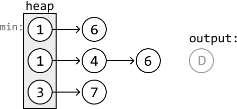
Keyin heap yordamida eng kichik qiymatli tugunni aniqlash va uni natija bog'liq ro'yxatiga qo'shish strategiyamizni amalga oshiramiz. Natija bog'liq ro'yxatini qurishda yordam berish uchun dummy tugundan foydalanamiz. Tugun olinib chiqarilgandan so'ng, uning bog'liq ro'yxatidagi keyingi tugun heap-ga qo'shiladi.
Heap bo'shagach, birlashtirilgan bog'liq ro'yxatning boshi bo'lgan dummy.next ni qaytarishimiz mumkin.
Amalga Oshirish
from typing import List
from ds import ListNode
import heapq

def combine_sorted_linked_lists(lists: List[ListNode]) -> ListNode:
    ListNode.__lt__ = lambda self, other: self.val < other.val
    heap = []
    for head in lists:
        if head:
            heapq.heappush(heap, head)
    dummy = ListNode(-1)
    curr = dummy
    while heap:
        smallest_node = heapq.heappop(heap)
        curr.next = smallest_node
        curr = curr.next
        if smallest_node.next:
            heapq.heappush(heap, smallest_node.next)
    return dummy.next
Murakkablik Tahlili
Vaqt murakkabligi: O(n log(k)), bu yerda n tugunlarning umumiy soni. Xotira murakkabligi: O(k).
Butun Sonlar Oqimining Medianasi
Butun Sonlar Oqimining Medianasi
Ma'lumotlar oqimidan butun sonlar qo'shish va istalgan vaqtda qabul qilingan barcha elementlarning medianasini qaytarishni qo'llab-quvvatlovchi ma'lumotlar strukturasini loyihalang.
- add(num: int) -> None: ma'lumotlar strukturasiga butun son qo'shadi.
- get_median() -> float: hozirgacha qabul qilingan barcha butun sonlarning medianasini qaytaradi.
Misol:
Input: [add(3), add(6), get_median(), add(1), get_median()]
Output: [4.5, 3.0]
Intuitsiya
Mediana doimo saralangan qiymatlar ro'yxatining o'rtasida joylashadi. Bu masaladagi qiyinlik — yangi qiymatlar kelganda barcha qiymatlarni saralangan holda saqlash noaniq.
Min-heap va max-heap kombinatsiyasidan foydalanishimiz mumkin:
- Max-heap chap yarmini boshqaradi, bu yerda tepadagi qiymat birinchi median qiymatini ifodalaydi.
- Min-heap o'ng yarmini boshqaradi, bu yerda tepadagi qiymat ikkinchi median qiymatini ifodalaydi.
Elementlarning umumiy soni toq bo'lsa, bitta mediana mavjud — bu medianani max-heap saqlashini belgilaymiz.
Heap-larni boshqarish uchun ikki qoida:
- Max-heap (chap yarmi) ning maksimal qiymati min-heap (o'ng yarmi) ning minimal qiymatidan kichik yoki teng bo'lishi kerak.
- Heap-lar teng hajmda bo'lishi kerak, lekin max-heap min-heap dan bitta ko'proq elementga ega bo'lishi mumkin.
Amalga Oshirish
import heapq

class MedianOfAnIntegerStream:
    def __init__(self):
        self.left_half = []   # max-heap (negated)
        self.right_half = []  # min-heap

    def add(self, num: int) -> None:
        if not self.left_half or num <= -self.left_half[0]:
            heapq.heappush(self.left_half, -num)
            if len(self.left_half) > len(self.right_half) + 1:
                heapq.heappush(self.right_half, -heapq.heappop(self.left_half))
        else:
            heapq.heappush(self.right_half, num)
            if len(self.right_half) > len(self.left_half):
                heapq.heappush(self.left_half, -heapq.heappop(self.right_half))

    def get_median(self) -> float:
        if len(self.left_half) == len(self.right_half):
            return (-self.left_half[0] + self.right_half[0]) / 2
        return float(-self.left_half[0])
Murakkablik Tahlili
add ning vaqt murakkabligi: O(log(n)). get_median ning vaqt murakkabligi: O(1). Xotira murakkabligi: O(n).
K-Saralangan Massivni Tartibga Solish
K-Saralangan Massivni Tartibga Solish
Har bir element saralangan pozitsiyasidan ko'pi bilan k ta o'rinda uzoqda bo'lgan butun sonlar massivi berilgan. Massivni kamaymaslik tartibida saralang.
Misol:
Input: nums = [5, 1, 9, 4, 7, 10], k = 2
Output: [1, 4, 5, 7, 9, 10]
Intuitsiya
K-saralangan massivda har bir element to'liq saralangan massivdagi o'rnidan ko'pi bilan k indeks uzoqda joylashadi.
Bu masalaning oddiy yechimi — standart saralash algoritmi yordamida massivni saralash. Ammo kirish ma'lumoti qisman saralangan (k-saralangan) bo'lganligi sababli, massivni saralashning tezroq usuli borligini taxmin qilishimiz kerak.
Istalgan i indeks uchun saralangan massivda i indeksiga tegishli element [i - k, i + k] oralig'ida joylashadi. 0 indeksida kerakli qiymat [0, 0 + k] oralig'idagi eng kichik sondir.
Bu yondashuvni yaxshilash uchun har bir [i, i + k] oralig'idagi minimal qiymatga samarali kirish uchun min-heap kerak.
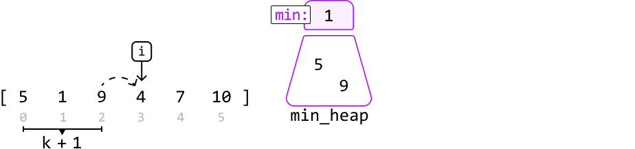
Amalga Oshirish
from typing import List
import heapq

def sort_a_k_sorted_array(nums: List[int], k: int) -> List[int]:
    min_heap = nums[:k+1]
    heapq.heapify(min_heap)
    insert_index = 0
    for i in range(k + 1, len(nums)):
        nums[insert_index] = heapq.heappop(min_heap)
        insert_index += 1
        heapq.heappush(min_heap, nums[i])
    while min_heap:
        nums[insert_index] = heapq.heappop(min_heap)
        insert_index += 1
    return nums
Murakkablik Tahlili
Vaqt murakkabligi: O(n log(k)). Xotira murakkabligi: O(k).
Intervallar
Intervallarga Kirish
Intervallarga Kirish
Intuitsiya
Interval ikki qiymatdan iborat: boshlang'ich nuqta va tugash nuqtasi. U son o'qida ushbu ikki nuqta orasidagi barcha qiymatlarni o'z ichiga oluvchi uzluksiz kesmani ifodalaydi. Ko'pincha chiziq, vaqt oralig'i yoki qiymatlarning uzluksiz diapazonini ifodalash uchun ishlatiladi.
- Intervalning boshlang'ich nuqtasi interval qayerdan boshlanishini bildiradi.
- Intervalning tugash nuqtasi interval qayerda tugashini bildiradi.

Intervallar yopiq, ochiq yoki yarim-ochiq bo'lishi mumkin — bu boshlang'ich yoki tugash nuqtalari intervalga kiritilgan-kiritilmaganligiga bog'liq.
- Yopiq intervallar: Boshlang'ich ham, tugash nuqtasi ham intervalga kiritilgan.

- Ochiq intervallar: Boshlang'ich ham, tugash nuqtasi ham intervalga kiritilmagan.

- Yarim-ochiq intervallar: Boshlang'ich yoki tugash nuqtalaridan biri kiritilgan, ikkinchisi esa kiritilmagan.

Suhbatda interval masalasi berilganda, intervallar yopiq, ochiq yoki yarim-ochiq ekanligini aniqlab olish muhim, chunki bu intervallarning qoplanish xarakterini o'zgartirishi mumkin.
Qoplanadigan intervallar Ikki interval kamida bitta umumiy qiymatni bo'lishsa, ular qoplanadi.
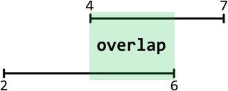
Ko'pchilik interval masalalarining asosiy qiyinligi — qoplanadigan intervalllarni samarali boshqarish. Qoplanadigan intervallarni aniqlash yoki birlashtirish bo'ladimi, intervallar o'rtasidagi qoplamaning masalaning kerakli natijasiga qanday ta'sir qilishini tushunish muhim. Ushbu bobdagi masalalar turli holatlarda qoplanadigan intervallarni boshqarishni o'z ichiga oladi.
Intervallarni saralash Ko'pchilik interval masalalarida muammoni hal qilishdan oldin intervallarni saralash juda foydali, chunki bu ularni ma'lum tartibda qayta ishlash imkonini beradi.
Odatda intervallarni boshlang'ich nuqtalari bo'yicha saralaymiz, shunda ular xronologik tartibda o'tkazilishi mumkin. Ikkita yoki undan ortiq intervalning boshlang'ich nuqtasi bir xil bo'lsa, saralashda har bir intervalning tugash nuqtalarini ham hisobga olishimiz kerak bo'lishi mumkin.
Boshlang'ich va tugash nuqtalarini ajratish Ba'zi holatlarda interval boshlang'ich va tugash nuqtalarini alohida qayta ishlash foydali bo'lishi mumkin. Bu odatda ikkita saralangan massiv yaratishni o'z ichiga oladi: biri barcha boshlang'ich nuqtalarni, ikkinchisi esa barcha tugash nuqtalarini o'z ichiga oladi. Masalan, bu Intervallarning Eng Katta Qoplamasi masalasida ko'riladigan sweeping line algoritmida kerak.

Interval klassi ta'rifi Bu bobdagi masalalar uchun intervallar quyidagi klass yordamida ifodalanadi.
class Interval:
   def __init__(self, start, end):
       self.start = start
       self.end = end
Hayotiy Misol
Rejalashtirish tizimlari: Intervallar rejalashtirish tizimlarida keng qo'llaniladi. Masalan, konferents-zal bron qilish tizimida har bir bron interval sifatida ifodalanadi. Interval ifodasidan foydalaniladi, agar tizim etarli xona mavjudligini ta'minlash uchun eng ko'p qoplanadigan bronlarni aniqlash kabi funksionallikni talab qilsa. Bu intervallarni tahlil qilib, tizim resurslarni samarali taqsimlashi va ikki marta bron qilishlarning oldini olishi mumkin.
Bob Rejasi
Qoplanadigan Intervallarni Birlashtirish
Qoplanadigan Intervallarni Birlashtirish
Intervallar massivini shunday birlashtiring, qoplanadigan intervallar qolmasin va birlashtirilgan intervalllarni qaytaring.
Misol:
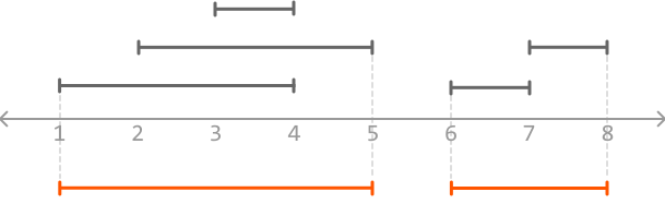
Input: intervals = [[3, 4], [7, 8], [2, 5], [6, 7], [1, 4]]
Output: [[1, 5], [6, 8]]
Cheklovlar:
- Kirish ma'lumoti kamida bitta intervaldan iborat.
- Massivdagi har bir i indeks uchun intervals[i].start ≤ intervals[i].end.
Intuitsiya
Bu masalaning ikkita asosiy qiyinligi:
- Qaysi intervallar bir-birini qoplashini aniqlash.
- O'sha intervallarni birlashtirish.
Keling, birinchi qiyinlikni hal qilishdan boshlaylik. A va B ikkita intervalini ko'rib chiqaylik, bu yerda A intervali B dan oldin boshlanadi. Quyida bu ikkita interval qoplanmaydigan holat tasvirlangan:
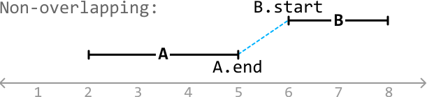
Yuqoridagi chiziqli chiziq A intervalining B boshlanishidan oldin tugashini ko'rsatadi, bu B ning A ni qoplash ehtimolini yo'q qiladi. Bu A va B intervallari A.end < B.start bo'lganda hech qachon qoplanmasligini bildiradi.
Endi bu ikkita intervalning qoplanadigan bir nechta holatini ko'rib chiqaylik:
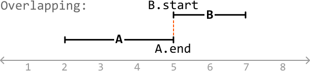
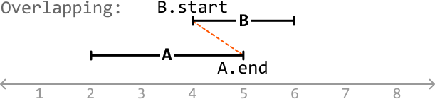
Bu hollarda B, A tugashidan oldin (yoki tugashida) boshlanadi (A.end ≥ B.start). Boshqacha aytganda, B ning bir qismi A bilan qoplanadi, chunki A intervali B boshlanishidan oldin tugamagan. Shuning uchun A.end ≥ B.start bo'lganda A va B intervallari qoplanadi.
Endi A intervalining B dan oldin boshlanishi shartida ikkala intervalning barcha qoplanadigan va qoplanmaydigan holatlarini qamrab oladigan ikki holat aniqlandi:
- Agar A.end < B.start bo'lsa, intervallar qoplanmaydi.
- Agar A.end ≥ B.start bo'lsa, intervallar qoplanadi.
Bu shartlarni kiritimdagi istalgan ikki intervalga qo'llash uchun qaysi interval birinchi boshlanishini aniqlash usuli foydali. Bir g'oya — intervallarni boshlang'ich qiymatlari bo'yicha saralash, bu har ikki qo'shni intervaldan qaysi biri birinchi boshlanishini aniq ko'rsatadi.
Intervallarni birlashtirish Yuqoridagi mantiq asosida keling, misolni ko'rib chiqaylik. Quyidagi intervallarni ko'rib chiqaylik:

Birinchi qadam — bu intervallarni boshlang'ich qiymati bo'yicha saralash:
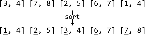
Tushuntirishga yordam berish uchun intervallarni vizual tarzda tasvirlaymiz:

Har bir intervallarni merged nomli yangi massivga qo'shamiz/birlashtiramiz. Birinchi intervaldan boshlaymiz — uni to'g'ridan-to'g'ri merged massiviga qo'shishimiz mumkin, chunki u birinchi interval:
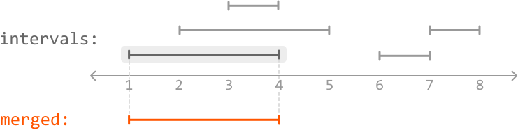
Birinchi interval qo'shilgandan so'ng, birlashtirish jarayonini boshlaymiz. A ni merged massivining oxirgi intervali, B ni esa kirish ma'lumotidagi joriy interval sifatida belgilaymiz.
B, A tugashidan oldin boshlanganini payqaymiz, bu qoplamani bildiradi. Keling, ularni birlashtiraylik:

A va B ni birlashtirish uchun ular orasidagi eng chap boshlang'ich qiymat va eng o'ng tugash qiymatidan foydalanamiz.
Keyingi intervalga ham xuddi shu mantiqni qo'llashimiz mumkin:

To'rtinchi intervalga yetganda B, A tugashidan keyin boshlanishini payqaymiz, bu qoplama yo'qligini bildiradi.

Shuning uchun uni merged massiviga yangi interval sifatida qo'shamiz:
Keyingi B intervali merged massivinining oxirgi A intervali bilan qoplanadi, chunki B, A tugashida boshlanadi (A.end == B.start).

Keling, A ni B bilan birlashtiraylik:
Oxirgi intervallar qayta ishlangandan so'ng, barcha intervallarni muvaffaqiyatli birlashtirdik.
Amalga Oshirish
from typing import List
from ds import Interval

def merge_overlapping_intervals(intervals: List[Interval]) -> List[Interval]:
    intervals.sort(key=lambda x: x.start)
    merged = [intervals[0]]
    for B in intervals[1:]:
        A = merged[-1]
        if A.end < B.start:
            merged.append(B)
        else:
            merged[-1] = Interval(A.start, max(A.end, B.end))
    return merged
Murakkablik Tahlili
Vaqt murakkabligi: saralash tufayli O(nlog(n)). Birlashtirish O(n) vaqt oladi.
Xotira murakkabligi: Python-ning Tim sort algoritmi uchun O(n).
Suhbat Maslahat
Maslahat: Mantiq va chekka holatlarni aniqlash uchun intervallarni vizuallashtiring. Misollar chizish suhbatdoshingizning fikringizni tushunishiga yordam beradi.
Barcha Interval Qoplamalarini Aniqlash
Barcha Interval Qoplamalarini Aniqlash
intervals1 va intervals2 bo'lgan ikki intervallar massivi orasidagi barcha qoplamalar massivini qaytaring. Har bir alohida interval massivi boshlang'ich qiymat bo'yicha saralangan va o'z ichida qoplanadigan intervallar mavjud emas.
Misol:

Input: intervals1 = [[1, 4], [5, 6], [9, 10]],
       intervals2 = [[2, 7], [8, 9]]
Output: [[2, 4], [5, 6], [9, 9]]
Cheklovlar:
- intervals1 dagi har bir i indeks uchun intervals1[i].start < intervals1[i].end.
- intervals2 dagi har bir j indeks uchun intervals2[j].start < intervals2[j].end.
Intuitsiya
Bizga ikki intervallar massivi berilgan, har birida qoplanadigan intervallar yo'q. Bu qoplama faqat birinchi massivdagi interval va ikkinchi massivdagi interval o'rtasida yuzaga kelishi mumkinligini bildiradi.
Ikkita qoplanadigan interval orasidagi qoplamani aniqlash Qoplanadigan Intervallarni Birlashtirish masalasidan bilamizki, A va B ikkita interval A, B dan oldin boshlanadi deb faraz qilinsa, A.end >= B.start bo'lganda qoplanadi.

Bu ikkita qoplanadigan interval orasidagi qoplamani ajratib olish uchun u qayerda boshlanishi va qayerda tugashini aniqlashimiz kerak.
- Qoplama eng uzoq boshlang'ich nuqtada boshlanadi, bu doimo B.start bo'ladi.
- Qoplama eng yaqin tugash nuqtasida tugaydi (min(A.end, B.end)).
Shuning uchun, ikkita interval qoplanishsa, ularning qoplamasi [B.start, min(A.end, B.end)] diapazoni bilan belgilanadi.
Barcha qoplamalarni aniqlash Endi ikki intervallar massiviga qaytaylik.

Har bir massivdan birinchi intervallarni ko'rib chiqishdan boshlaylik:

Bu intervallarning qoplanadigan-qoplanmasligini tekshirish uchun qaysi interval birinchi boshlanishini aniqlaymiz, uni A sifatida, ikkinchisini B sifatida belgilaymiz:
if intervals1[i].start <= intervals2[j].start:
    A, B = intervals1[i], intervals2[j]
else:
    A, B = intervals2[j], intervals1[i]
![Image represents intervals1[i] starting first, labelled A.](https://bytebytego.com/images/courses/coding-patterns/intervals/identify-all-interval-overlaps/image-09-02-5-6FYA5HUP.svg?dpl=dpl_Gs7zfM6MUzjTBjcjps1LqXtb9QmD)
A va B, A.end >= B.start bo'lganda qoplanadi, bu yerda bu to'g'ri. Qoplamani yozib olamiz: [B.start, min(A.end, B.end)]:
Qoplamani aniqlagandan so'ng, birinchi tugaydigan intervalning ko'rsatkichini oldinga siljiting.
![Image represents advancing pointer i after intervals1[i] ends before intervals2[j].](https://bytebytego.com/images/courses/coding-patterns/intervals/identify-all-interval-overlaps/image-09-02-7-XEMGOSPW.svg?dpl=dpl_Gs7zfM6MUzjTBjcjps1LqXtb9QmD)
Endi interval massivlarini o'tayotganda barcha qoplamalarni aniqlash va yozib olish imkonini beruvchi jarayonni aniqladik:
- A ni birinchi boshlanadigan interval, B ni esa ikkinchisi sifatida belgilang.
- Bu intervallarning qoplanadigan-qoplanmasligini ko'rish uchun A.end >= B.start ni tekshiring. Agar qoplansa, qoplamani [B.start, min(A.end, B.end)] sifatida yozib oling.
- Birinchi tugaydigan intervalning mos ko'rsatkichini keyingi intervalga o'tish uchun oldinga siljiting.
i yoki j o'z massivining oxiriga yetguncha davom eting.
Amalga Oshirish
from typing import List
from ds import Interval

def identify_all_interval_overlaps(intervals1: List[Interval], intervals2: List[Interval]) -> List[Interval]:
   overlaps = []
   i = j = 0
   while i < len(intervals1) and j < len(intervals2):
       if intervals1[i].start <= intervals2[j].start:
           A, B = intervals1[i], intervals2[j]
       else:
           A, B = intervals2[j], intervals1[i]
       if A.end >= B.start:
           overlaps.append(Interval(B.start, min(A.end, B.end)))
       if intervals1[i].end < intervals2[j].end:
           i += 1
       else:
           j += 1
   return overlaps
Murakkablik Tahlili
Vaqt murakkabligi: O(n+m), bu yerda n va m intervals1 va intervals2 uzunliklari.
Xotira murakkabligi: O(1).
Intervallarning Eng Katta Qoplamasi
Intervallarning Eng Katta Qoplamasi
Intervallar massivi berilgan. Istalgan nuqtada qoplanadigan intervallarning maksimal sonini aniqlang. Har bir interval yarim-ochiq, ya'ni boshlang'ich nuqtani o'z ichiga oladi, ammo tugash nuqtasini olmaydi.
Misol:
Input: intervals = [[1, 3], [5, 7], [2, 6], [4, 8]]
Output: 3
Cheklovlar:
- Kirish ma'lumoti kamida bitta intervaldan iborat bo'ladi.
- Ro'yxatdagi har bir i indeks uchun intervals[i].start < intervals[i].end.
Intuitsiya
Ma'lum bir vaqt nuqtasida x ta interval qoplanishi nima anglatishini o'ylab ko'ring. Bu shu nuqtada x ta 'faol' interval mavjudligini bildiradi, ya'ni interval boshlangan, lekin hali tugamagan.
Quyidagi misolda 5-vaqtda uchta faol intervalga ega ekanligimizni ko'ramiz:
Istalgan vaqt nuqtasida faol intervallar sonini topish uchun interval qachon boshlangan va qachon tugaganini aniqlashimiz kerak. Boshlang'ich nuqta yangi faol intervalning boshlanishini, tugash nuqtasi esa faol intervalning tugashini bildiradi.
Boshlang'ich va tugash nuqtalarini qayta ishlash Keling, har bir nuqtani xronologik tartibda o'taylik va har nuqtada faol intervallar sonini aniqlaymiz.
Birinchi nuqta — boshlang'ich nuqta, hisoblagichimizni oshiradi:

Keyingi nuqta yana boshlang'ich nuqta, hisoblagichni 2 ga oshiradi:

Keyingi nuqta — tugash nuqtasi, hisoblagichni 1 ga kamaytiradi:

Har bir nuqta turida nima qilish kerakligini asosladik:
- Boshlang'ich nuqtaga duch kelsak: active_intervals ni oshiring.
- Tugash nuqtasiga duch kelsak: active_intervals ni kamaytiring.
Yakuniy javob active_intervals ning eng katta qiymati kuzatib borilishi orqali olinadi.
Chekka holat: bir vaqtdagi boshlang'ich va tugash nuqtalarini qayta ishlash Boshlang'ich va tugash nuqtasi bir vaqtda sodir bo'lganda, tugash nuqtalarini boshlang'ich nuqtalardan oldin qayta ishlashimiz kerak — shunda yeni tugagan intervalni faol sifatida sanashdan saqlanamiz.

Tugash nuqtasini birinchi qayta ishlasak, bu muammoga duch kelmaymiz:

Shuning uchun, bir vaqtda sodir bo'ladigan boshlang'ich va tugash nuqtalari uchun tugash nuqtalarini boshlang'ich nuqtalardan oldin qayta ishlang.
Interval nuqtalarini tartibda o'tish Barcha boshlang'ich va tugash nuqtalarini bitta massivga birlashtiring, uni saralang va teng qiymatlar uchun tugash nuqtalarini boshlang'ich nuqtalardan oldin qo'yishni ta'minlang.
Bu masalani hal qilish uchun ishlatgan algoritmimiz 'sweeping line algoritmi' nomi bilan tanilgan. U vertikal chiziq ularni kesib o'tayotganday, interval boshlang'ich va tugash nuqtalarini tartib bilan qayta ishlash orqali ishlaydi.
Amalga Oshirish
from typing import List
from ds import Interval

def largest_overlap_of_intervals(intervals: List[Interval]) -> int:
   points = []
   for interval in intervals:
       points.append((interval.start, 'S'))
       points.append((interval.end, 'E'))
   points.sort(key=lambda x: (x[0], x[1]))
   active_intervals = 0
   max_overlaps = 0
   for time, point_type in points:
       if point_type == 'S':
           active_intervals += 1
       else:
           active_intervals -= 1
       max_overlaps = max(max_overlaps, active_intervals)
   return max_overlaps
Murakkablik Tahlili
Vaqt murakkabligi: 2n o'lchamli points massivini saralash tufayli O(n*log(n)).
Xotira murakkabligi: points massivi tufayli O(n).
Prefiks Yig'indilar
Prefiks Yig'indilarga Kirish
Prefiks Yig'indilarga Kirish
Intuitsiya
Bir necha kun davomida tashqarida ovqatlanishga sarflagan pullaringizni kuzatib borishingizni tasavvur qiling.
![Image represents spendings list = [10, 15, 20, 10, 5] aligned with days Mon-Fri.](https://bytebytego.com/images/courses/coding-patterns/prefix-sums/introduction-to-prefix-sums/image-10-00-1-WDTVKAVE.svg?dpl=dpl_Gs7zfM6MUzjTBjcjps1LqXtb9QmD)
Prefiks yig'indi massivi massivdagi har bir indeksgacha bo'lgan qiymatlarning yig'indi summasini saqlaydi. Chorshanba kunigacha sarflangan jami summa $45 ($10+$15+$20).
![Image represents spendings [10,15,20,10,5] and prefix_sums [10,25,45,55,60] arrays aligned with Mon-Fri.](https://bytebytego.com/images/courses/coding-patterns/prefix-sums/introduction-to-prefix-sums/image-10-00-2-2QJ5YCRR.svg?dpl=dpl_Gs7zfM6MUzjTBjcjps1LqXtb9QmD)
Har bir indeksdagi prefiks yig'indini olish uchun kiritish massividagi joriy sonni oldingi indeksdagi prefiks yig'indisiga qo'shing.
![Image represents step-by-step calculation of prefix sums for array [10,15,20,10,5].](https://bytebytego.com/images/courses/coding-patterns/prefix-sums/introduction-to-prefix-sums/image-10-00-3-TNX4KXVG.svg?dpl=dpl_Gs7zfM6MUzjTBjcjps1LqXtb9QmD)
Kodda yuqoridagi jarayon quyidagicha ko'rinadi:
def compute_prefix_sums(nums):
    prefix_sum = [nums[0]]
    for i in range(1, len(nums)):
        prefix_sum.append(prefix_sum[-1] + nums[i])
Prefiks yig'indi massivini qurish O(n) vaqt va O(n) xotira talab qiladi, bunda n massiv uzunligini bildiradi.
Prefiks yig'indilarning qo'llanilishi Doimiy vaqtda yig'indi summalariga kirish imkonidan tashqari, prefiks yig'indilar qism massivlar yig'indisini samarali hisoblashda keng qo'llaniladi. Yana bir qiziqarli variant — prefiks ko'paytmalar bo'lib, u yig'indilar o'rniga kumulyativ ko'paytmani massivga saqlaydi.
Haqiqiy Hayotdagi Misol
Moliyaviy tahlil: Prefiks yig'indilarning real hayotdagi foydalanishi — moliyaviy tahlil, ayniqsa vaqt bo'yicha kumulyativ daromad yoki xarajatlarni hisoblashda. Prefiks yig'indilarni oldindan hisoblab, kompaniya har kuni alohida daromadni qo'shmasdan, istalgan davr uchun daromadni darhol aniqlay oladi.
Bob Bo'lim Mazmuni
Oraliq Yig'indisi
Oraliq Yig'indisi
Butun sonlar massivi berilgan bo'lsa, ikki indeks orasidagi qiymatlar yig'indisini qaytaruvchi funksiya yozing.
Misol:
![Image represents three examples of sum_range function on [3, -7, 6, 0, -2, 5].](https://bytebytego.com/images/courses/coding-patterns/prefix-sums/sum-between-range/sum-between-range-YTKLP363.svg?dpl=dpl_Gs7zfM6MUzjTBjcjps1LqXtb9QmD)
Input: nums = [3, -7, 6, 0, -2, 5],
       [sum_range(0, 3), sum_range(2, 4), sum_range(2, 2)]
Output: [2, 4, 6]
Cheklovlar:
- nums kamida bitta elementni o'z ichiga oladi.
- Har bir sum_range operatsiyasi kiritish massivining to'g'ri oralig'ini so'raydi.
Intuitsiya
sum_range(i, j) funksiyasini kodlashimiz kerak. Sodda yechim har chaqiruvda i dan j gacha iterativ ravishda yig'indi hisoblab, chiziqli vaqt sarflaydi. Prefiks yig'indilardan foydalanish samaradorlikni oshiradi.
Butun sonlar massivi va uning prefiks yig'indisini ko'rib chiqing:
![Image represents nums [3,-7,6,0,-2,5] and prefix_sum [3,-4,2,2,0,5] arrays.](https://bytebytego.com/images/courses/coding-patterns/prefix-sums/sum-between-range/image-10-01-1-VMKJURRC.svg?dpl=dpl_Gs7zfM6MUzjTBjcjps1LqXtb9QmD)
Har qanday j indeksgacha bo'lgan prefiks yig'indi sum_range(0, j) javobini beradi. Masalan, [0, 3] oralig'ining yig'indisi prefix_sum[3] ga teng.
Shuning uchun, i == 0 bo'lganda:
sum_range(0, j) = prefix_sum[j]
[2, 4] oralig'i uchun yig'indi prefix_sum[4] - prefix_sum[1] ga teng:
![Image represents subarray [6, 0, -2] within [3,-7,6,0,-2,5].](https://bytebytego.com/images/courses/coding-patterns/prefix-sums/sum-between-range/image-10-01-3-H55BHFLR.svg?dpl=dpl_Gs7zfM6MUzjTBjcjps1LqXtb9QmD)
![Image represents sum[0:4] highlighted in the array.](https://bytebytego.com/images/courses/coding-patterns/prefix-sums/sum-between-range/image-10-01-4-BKFCNYT4.svg?dpl=dpl_Gs7zfM6MUzjTBjcjps1LqXtb9QmD)
[2, 4] oralig'i yig'indisi = prefix_sum[4] - prefix_sum[1], ya'ni [0, 4] yig'indisidan [0, 1] yig'indisini ayirish.
![Image represents sum[2:4] = sum[0:4] - sum[0:1] visualization.](https://bytebytego.com/images/courses/coding-patterns/prefix-sums/sum-between-range/image-10-01-5-BSWFQB25.svg?dpl=dpl_Gs7zfM6MUzjTBjcjps1LqXtb9QmD)
Shuning uchun, i > 0 bo'lganda:
sum_range(i, j) = prefix_sum[j] - prefix_sum[i - 1]
Amalga Oshirish
from typing import List

class SumBetweenRange:
    def __init__(self, nums: List[int]):
        self.prefix_sum = [nums[0]]
        for i in range(1, len(nums)):
            self.prefix_sum.append(self.prefix_sum[-1] + nums[i])

    def sum_range(self, i: int, j: int) -> int:
        if i == 0:
            return self.prefix_sum[j]
        return self.prefix_sum[j] - self.prefix_sum[i - 1]
Murakkablik Tahlili
Vaqt murakkabligi: Konstruktor O(n). sum_range O(1).
Xotira murakkabligi: prefix_sum massivi uchun O(n).
K-Yig'indili Qism Massivlar
K-Yig'indili Qism Massivlar
Butun sonlar massivida yig'indisi k ga teng bo'lgan qism massivlar sonini toping.
Misol:
![Image represents three subarrays of [1,2,-1,1,2] that sum to 3.](https://bytebytego.com/images/courses/coding-patterns/prefix-sums/k-sum-subarrays/k-sum-subarrays-SGSPMDU3.svg?dpl=dpl_Gs7zfM6MUzjTBjcjps1LqXtb9QmD)
Input: nums = [1, 2, -1, 1, 2], k = 3
Output: 3
Intuitsiya
Qo'pol kuch yechimi har bir mumkin bo'lgan qism massivni O(n^3) vaqtda tekshiradi. Prefiks yig'indilardan foydalanish buni kamaytiradi.
[i,j] qism massivining yig'indisi = prefix_sum[j] - prefix_sum[i-1] (i>0 bo'lganda), yoki faqat prefix_sum[j] (i=0 bo'lganda).

![Image represents prefix_sum[j] = sum[0:j].](https://bytebytego.com/images/courses/coding-patterns/prefix-sums/k-sum-subarrays/image-10-02-2-26EJOFO6.svg?dpl=dpl_Gs7zfM6MUzjTBjcjps1LqXtb9QmD)
Har ikkala holatni birlashtirish uchun prefiks yig'indilar massivi boshiga 0 qo'shamiz, shu tariqa i=0 bo'lganda ham prefix_sum[i-1]=0 amal qiladi.
![Image represents prefix_sums [0,1,3,2,3,5] with leading 0 prepended.](https://bytebytego.com/images/courses/coding-patterns/prefix-sums/k-sum-subarrays/image-10-02-3-IUWBVKVV.svg?dpl=dpl_Gs7zfM6MUzjTBjcjps1LqXtb9QmD)
from typing import List

def k_sum_subarrays(nums: List[int], k: int) -> int:
    n = len(nums)
    count = 0
    prefix_sum = [0]
    for i in range(0, n):
        prefix_sum.append(prefix_sum[-1] + nums[i])
    for j in range(1, n + 1):
        for i in range(1, j + 1):
            if prefix_sum[j] - prefix_sum[i - 1] == k:
                count += 1
    return count
Bu O(n^2) yechimni xesh-map yordamida optimallashtirish mumkin. Har bir prefiks yig'indi (curr_prefix_sum) uchun avval curr_prefix_sum - k necha marta uchraganini toping.

Har bir element uchun curr_prefix_sum - k xesh-mapda bor-yo'qligini tekshiring. Topilsa, uning chastotasini countga qo'shing.


Strategiya: 1) curr_prefix_sum ni yangilang. 2) curr_prefix_sum-k mapda bo'lsa, chastotasini countga qo'shing. 3) curr_prefix_sum ni mapga qo'shing.



Amalga Oshirish
from typing import List

def k_sum_subarrays_optimized(nums: List[int], k: int) -> int:
    count = 0
    prefix_sum_map = {0: 1}
    curr_prefix_sum = 0
    for num in nums:
        curr_prefix_sum += num
        if curr_prefix_sum - k in prefix_sum_map:
            count += prefix_sum_map[curr_prefix_sum - k]
        prefix_sum_map[curr_prefix_sum] = prefix_sum_map.get(curr_prefix_sum, 0) + 1
    return count
Murakkablik Tahlili
Vaqt murakkabligi: O(n) — nums bo'yicha bir marta iteratsiya.
Xotira murakkabligi: Xesh-map uchun O(n).
Joriy Element Siz Mahsulotlar Massivi
Joriy Element Siz Mahsulotlar Massivi
Butun sonlar massivi berilgan bo'lsa, res[i] nums[i] dan tashqari barcha elementlarning ko'paytmasiga teng bo'lgan res massivini qaytaring.
Misol:
Input: nums = [2, 3, 1, 4, 5]
Output: [60, 40, 120, 30, 24]
Tushuntirish: 0-indeksdagi chiqish qiymati nums[0] dan tashqari barcha sonlarning ko'paytmasi (3*1*4*5 = 60).
Intuitsiya
Oddiy yechim jami ko'paytmani har bir elementga bo'ladi (jami=120). Ammo bo'lish taqiqlansa nima bo'ladi?
![Image represents total product 120 divided by each element to produce res=[60,40,120,30,24].](https://bytebytego.com/images/courses/coding-patterns/prefix-sums/product-array-without-current-element/image-10-03-1-N4GBWUNI.svg?dpl=dpl_Gs7zfM6MUzjTBjcjps1LqXtb9QmD)
Bo'lishsiz, har qanday indeks uchun chiqish = chap tomonidagi barcha sonlar ko'paytmasi * o'ng tomonidagi barcha sonlar ko'paytmasi.
![Image represents res[i] = left_product * right_product visualization.](https://bytebytego.com/images/courses/coding-patterns/prefix-sums/product-array-without-current-element/image-10-03-2-4VEDNKPP.svg?dpl=dpl_Gs7zfM6MUzjTBjcjps1LqXtb9QmD)
Bizga ikki massiv kerak:
- left_products: left_products[i] — i ning chap tomonidagi barcha qiymatlar ko'paytmasi.
- right_products: right_products[i] — i ning o'ng tomonidagi barcha qiymatlar ko'paytmasi.
![Image represents left_products [1,2,6,6,24] and right_products [60,20,20,5,1] calculated from nums.](https://bytebytego.com/images/courses/coding-patterns/prefix-sums/product-array-without-current-element/image-10-03-3-VYSSWNKT.svg?dpl=dpl_Gs7zfM6MUzjTBjcjps1LqXtb9QmD)
Prefiks ko'paytmalar Prefiks ko'paytmalar kumulyativ ko'paytirishni ishlatadi (0 o'rniga 1 bilan initsializatsiya qilinadi).
- Kumulyativ qo'shish o'rniga kumulyativ ko'paytirish ishlatiladi.
- Prefiks ko'paytmalar massivi 0 o'rniga 1 bilan initsializatsiya qilinadi.
![Image represents left_products initialized with [1].](https://bytebytego.com/images/courses/coding-patterns/prefix-sums/product-array-without-current-element/image-10-03-4-DZZMAPDB.svg?dpl=dpl_Gs7zfM6MUzjTBjcjps1LqXtb9QmD)
![Image represents left_products = [1,2] after first multiplication.](https://bytebytego.com/images/courses/coding-patterns/prefix-sums/product-array-without-current-element/image-10-03-5-HHXGSRBD.svg?dpl=dpl_Gs7zfM6MUzjTBjcjps1LqXtb9QmD)
![Image represents left_products = [1,2,6] after second multiplication.](https://bytebytego.com/images/courses/coding-patterns/prefix-sums/product-array-without-current-element/image-10-03-6-3NKFAYMJ.svg?dpl=dpl_Gs7zfM6MUzjTBjcjps1LqXtb9QmD)
![Image represents left_products = [1,2,6,6,1] partially filled.](https://bytebytego.com/images/courses/coding-patterns/prefix-sums/product-array-without-current-element/image-10-03-7-5RVNNOFE.svg?dpl=dpl_Gs7zfM6MUzjTBjcjps1LqXtb9QmD)
![Image represents left_products = [1,2,6,6,24] complete.](https://bytebytego.com/images/courses/coding-patterns/prefix-sums/product-array-without-current-element/image-10-03-8-4SC67TAJ.svg?dpl=dpl_Gs7zfM6MUzjTBjcjps1LqXtb9QmD)
right_products o'ngdan chapga shunga o'xshash quriladi. Har ikkala massiv tayyor bo'lgach, res[i] = left_products[i] * right_products[i].

![Image represents right_products first step [5,1].](https://bytebytego.com/images/courses/coding-patterns/prefix-sums/product-array-without-current-element/image-10-03-10-YCIVOIZO.svg?dpl=dpl_Gs7zfM6MUzjTBjcjps1LqXtb9QmD)
![Image represents right_products = [20,5,1] partially filled.](https://bytebytego.com/images/courses/coding-patterns/prefix-sums/product-array-without-current-element/image-10-03-11-CY3FIWS6.svg?dpl=dpl_Gs7zfM6MUzjTBjcjps1LqXtb9QmD)
![Image represents right_products = [20,20,5,1] partially filled.](https://bytebytego.com/images/courses/coding-patterns/prefix-sums/product-array-without-current-element/image-10-03-12-4URC62ZT.svg?dpl=dpl_Gs7zfM6MUzjTBjcjps1LqXtb9QmD)
![Image represents right_products = [60,20,20,5,1] complete.](https://bytebytego.com/images/courses/coding-patterns/prefix-sums/product-array-without-current-element/image-10-03-13-XNC7B4L7.svg?dpl=dpl_Gs7zfM6MUzjTBjcjps1LqXtb9QmD)
Xotirani kamaytirish: res ni avval chap ko'paytmalar bilan to'ldiring, so'ng o'ngdan chapga aylanuvchi right_product bilan o'rinda ko'paytiring.
![Image represents res populated with left products [1,2,6,6,24].](https://bytebytego.com/images/courses/coding-patterns/prefix-sums/product-array-without-current-element/image-10-03-14-JGVIF7K3.svg?dpl=dpl_Gs7zfM6MUzjTBjcjps1LqXtb9QmD)
![Image represents res[i] = 6 * 20 = 120 at index 2.](https://bytebytego.com/images/courses/coding-patterns/prefix-sums/product-array-without-current-element/image-10-03-16-R7U4TU72.svg?dpl=dpl_Gs7zfM6MUzjTBjcjps1LqXtb9QmD)
![Image represents res[i] = 2 * 20 = 40 at index 1.](https://bytebytego.com/images/courses/coding-patterns/prefix-sums/product-array-without-current-element/image-10-03-17-KGXPQAXO.svg?dpl=dpl_Gs7zfM6MUzjTBjcjps1LqXtb9QmD)
![Image represents final res = [60,40,120,30,24].](https://bytebytego.com/images/courses/coding-patterns/prefix-sums/product-array-without-current-element/image-10-03-18-F3DT7OCI.svg?dpl=dpl_Gs7zfM6MUzjTBjcjps1LqXtb9QmD)
Amalga Oshirish
from typing import List

def product_array_without_current_element(nums: List[int]) -> List[int]:
    n = len(nums)
    res = [1] * n
    for i in range(1, n):
        res[i] = res[i - 1] * nums[i - 1]
    right_product = 1
    for i in range(n - 1, -1, -1):
        res[i] *= right_product
        right_product *= nums[i]
    return res
Murakkablik Tahlili
Vaqt murakkabligi: O(n) — nums bo'yicha ikki marta iteratsiya.
Xotira murakkabligi: O(1). res massivi xotira murakkabligi tahlilida hisobga olinmaydi.
Daraxtlar
Daraxtlarga Kirish
Daraxtlarga Kirish
Intuitsiya
Daraxt — tugunlardan tashkil topgan ierarxik ma'lumotlar tuzilmasi bo'lib, har bir tugun bir yoki bir nechta bolalar tugunlarga ulanadi. Daraxtdagi har bir tugun saqlaydigan ma'lumotni (val) va bolalar tugunlarga havolalarni o'z ichiga oladi. Eng keng tarqalgan daraxt turi — ikkilik daraxt bo'lib, unda har bir tugun ko'pi bilan ikkita bolaga ulanadi: chap bola va o'ng bola.
Quyida TreeNode klassining amalga oshirilishi keltirilgan:
class TreeNode:
    def __init__(self, val):
        self.val = val
        self.left = None
        self.right = None
Atamalar:
- Ota-tugun: bir yoki bir nechta bolaga ega tugun.
- Bola-tugun: ota-tugunga ega tugun.
- Pastki daraxt: tugun va uning avlodlaridan tashkil topgan daraxt.
- Yo'l: qirralar bilan bog'langan tugunlarning uzluksiz ketma-ketligi.
- Chuqurlik: ildizdan berilgan tugunga qadar bo'lgan qirralar soni.
Daraxt atributlari:
- Ildiz: daraxtning eng yuqori tuguniy va otasi bo'lmagan yagona tugun.
- Oraliq tugun: ota-tugunga va kamida bitta bolaga ega tugun.
- Barg: bolalari bo'lmagan tugun.
- Qirra: ikki tugunni bog'laydigan aloqa. Daraxtlarda odatda yo'naltirilgan qirralar bo'ladi, ya'ni qirralar faqat ota-tugundan bolaga yo'nalgan bo'ladi.
- Balandlik: ildizdan bargga qadar bo'lgan eng uzun yo'l uzunligi.1
Quyidagi muhokamada biz asosan ikkilik daraxtlarga e'tibor qaratamiz.
Daraxt O'tishlari
Chuqurlik-birinchi qidiruv (DFS) DFS — daraxtning barcha tugunlarini ko'rib chiqish usuli bo'lib, ildizdan boshlab mumkin qadar chuqur sho'ng'ib boradi, keyin boshqa tarmoqlarni ko'rib chiqish uchun orqaga qaytadi.
DFS odatda rekursiv tarzda amalga oshiriladi:
def dfs(node: TreeNode):
    if node is None:
        return
    process(node)       # Joriy tugunni qayta ishlash.
    dfs(node.left)      # Chap pastki daraxtni o'tish.
    dfs(node.right)     # O'ng pastki daraxtni o'tish.
Yuqoridagi rekursiv amalga oshirish oldindan tartibli (preorder) o'tish tartibiga mos keladi. DFSning yana ikkita keng tarqalgan usuli — tartibli (inorder) va keyingi tartibli (postorder) o'tish. Farqi quyidagicha:
DFS ko'plab foydalanish holatlari bo'lib, daraxtni o'tishda eng keng tarqalgan tanlov.
- Oldindan tartibli o'tish — DFS o'tishining eng keng tarqalgan turi. Shuningdek, har bir pastki daraxtning ildiz tugunini bolalardan oldin qayta ishlash kerak bo'lganda ishlatiladi.
- Tartibli o'tish — daraxt tugunlarini chapdan o'ngga qarab qayta ishlash kerak bo'lganda ishlatiladi.
- Keyingi tartibli o'tish — kamroq ishlatiladigan o'tish usuli, ammo har bir tugunning pastki daraxtlari ildizidan oldin qayta ishlanishi kerak bo'lganda muhim.
Ushbu bobdagi masalalar DFSning foydalanish holatlarini batafsil ko'rib chiqadi va bu o'tish usullarini qachon va qanday qo'llashning amaliy misollarini beradi.
Kenglik-birinchi qidiruv (BFS) BFS daraxt tugunlarini daraja bo'yicha o'tadi. Joriy darajadagi tugunlarni qayta ishlab, keyin keyingi chuqurlik darajasidagi tugunlarga o'tadi.
def bfs(root: TreeNode):
    if root is None:
        return
    queue = deque([root])
    while queue:
        node = queue.popleft()
        process(node)  # Joriy tugunni qayta ishlash.
        if node.left:
            queue.append(node.left)  # Chap bolani navbatga qo'shish.
        if node.right:
            queue.append(node.right)  # O'ng bolani navbatga qo'shish.
BFS daraxtda ma'lum bir manzilga eng qisqa yo'lni topishda yoki daraxtni daraja bo'yicha qayta ishlashda keng qo'llaniladi. O'tish paytida har bir tugunning aniq darajasini bilish muhim bo'lganda, darajali tartibli o'tish (level-order traversal) deb ataladigan BFS varianti ishlatiladi.
Murakkablik tavsifi Quyida n daraxtdagi tugunlar sonini, h esa daraxt balandligini bildiradi.
Haqiqiy Hayotdagi Misol
Fayl tizimlari: Ko'pgina operatsion tizimlarda fayl tizimi ierarxik daraxt tuzilmasi sifatida tashkil etilgan. Ildiz katalogi daraxtning ildizi bo'lib, tizimdagi har bir fayl yoki papka tugundir. Papkalar pastki papkalar yoki fayllarni bola tugunlar sifatida o'z ichiga olishi mumkin. Kompyuterda papkalar bo'yicha o'tayotganingizda, aslida daraxt tuzilmasini navigatsiya qilayapiz.
Bob Bo'lim Mazmuni
E'tibor bering, DFS ostida sanab o'tilgan ba'zi masalalar BFS yoki boshqa o'tish algoritmlari bilan ham yechilishi mumkin. Xuddi shu narsa BFS ostidagi masalalar uchun ham amal qiladi.
Izohlar
- Ba'zi manbalar daraxt balandligini boshqacha belgilashi mumkin. Ushbu kitobda rekursiv algoritmlarni loyihalashni yanada intuitiv qiluvchi ta'rifdan foydalanamiz. Bu yerda faqat bitta tugunga ega daraxt balandligi 1 deb hisoblanadi. ↩
Ikkilik Daraxtni Teskari Aylantirish
Ikkilik Daraxtni Teskari Aylantirish
Ikkilik daraxtni teskari aylantiring va uning ildizini qaytaring. Ikkilik daraxt teskari aylantirilganda, u o'zining ko'zgu tasviriga aylanadi.
Misol:
Intuitsiya - Rekursiv
Ikkilik daraxtni teskari aylantirish — aslida daraxtni vertikal o'q bo'yicha "ag'darish".
from ds import TreeNode

def invert_binary_tree_recursive(root: TreeNode) -> TreeNode:
    if not root:
        return None
    root.left, root.right = root.right, root.left
    invert_binary_tree_recursive(root.left)
    invert_binary_tree_recursive(root.right)
    return root
Amalga Oshirish - Iterativ
from ds import TreeNode

def invert_binary_tree_iterative(root: TreeNode) -> TreeNode:
    if not root:
        return None
    stack = [root]
    while stack:
        node = stack.pop()
        node.left, node.right = node.right, node.left
        if node.left:
            stack.append(node.left)
        if node.right:
            stack.append(node.right)
    return root
Muvozanatli Ikkilik Daraxtni Tekshirish
Muvozanatli Ikkilik Daraxtni Tekshirish
Ikkilik daraxtning balandlik bo'yicha muvozanatli ekanligini aniqlang, ya'ni hech bir tugunning chap va o'ng pastki daraxtlari balandligi farqi 1 dan oshmasin.
from ds import TreeNode

def balanced_binary_tree_validation(root: TreeNode) -> bool:
    return get_height_imbalance(root) != -1

def get_height_imbalance(node: TreeNode) -> int:
    if not node:
        return 0
    left_height = get_height_imbalance(node.left)
    right_height = get_height_imbalance(node.right)
    if left_height == -1 or right_height == -1:
        return -1
    if abs(left_height - right_height) > 1:
        return -1
    return 1 + max(left_height, right_height)
Ikkilik Daraxtning O'ng Tomonidagi Tugunlar
Ikkilik Daraxtning O'ng Tomonidagi Tugunlar
Ikkilik daraxtning har bir darajasidagi eng o'ng tugunlar qiymatlarini o'z ichiga olgan massiv qaytaring.
from ds import TreeNode

def rightmost_nodes_of_a_binary_tree(root: TreeNode) -> List[int]:
    if not root:
        return []
    res = []
    queue = deque([root])
    while queue:
        level_size = len(queue)
        for i in range(level_size):
            node = queue.popleft()
            if node.left:
                queue.append(node.left)
            if node.right:
                queue.append(node.right)
            if i == level_size - 1:
                res.append(node.val)
    return res
Ikkilik Daraxtning Eng Keng Darajasi
Ikkilik Daraxtning Eng Keng Darajasi
Ikkilik daraxtdagi eng keng darajaning kengligi qaytaring, bunda darajaning kengligi uning eng chap va eng o'ng null bo'lmagan tugunlari orasidagi masofa sifatida aniqlanadi.
from ds import TreeNode

def widest_binary_tree_level(root: TreeNode) -> int:
    if not root:
        return 0
    max_width = 0
    queue = deque([(root, 0)])
    while queue:
        level_size = len(queue)
        leftmost_index = queue[0][1]
        rightmost_index = leftmost_index
        for _ in range(level_size):
            node, i = queue.popleft()
            if node.left:
                queue.append((node.left, 2*i + 1))
            if node.right:
                queue.append((node.right, 2*i + 2))
            rightmost_index = i
        max_width = max(max_width, rightmost_index - leftmost_index + 1)
    return max_width
Ikkilik Qidiruv Daraxtini Tekshirish
Ikkilik Qidiruv Daraxtini Tekshirish
Ikkilik daraxtning to'g'ri ikkilik qidiruv daraxti (BST) ekanligini tekshiring.
from ds import TreeNode

def binary_search_tree_validation(root: TreeNode) -> bool:
    return is_within_bounds(root, float('-inf'), float('inf'))

def is_within_bounds(node: TreeNode, lower_bound: int, upper_bound: int) -> bool:
    if not node:
        return True
    if not lower_bound < node.val < upper_bound:
        return False
    if not is_within_bounds(node.left, lower_bound, node.val):
        return False
    return is_within_bounds(node.right, node.val, upper_bound)
Eng Quyi Umumiy Ajdod
Eng Quyi Umumiy Ajdod
Ikkilik daraxtdagi p va q ikki tugunning eng quyi umumiy ajdodini (LCA) qaytaring.
from ds import TreeNode

def lowest_common_ancestor(root: TreeNode, p: TreeNode, q: TreeNode) -> TreeNode:
    dfs(root, p, q)
    return lca

def dfs(node: TreeNode, p: TreeNode, q: TreeNode) -> bool:
    global lca
    if not node:
        return False
    node_is_p_or_q = node == p or node == q
    left_contains_p_or_q = dfs(node.left, p, q)
    right_contains_p_or_q = dfs(node.right, p, q)
    if node_is_p_or_q + left_contains_p_or_q + right_contains_p_or_q == 2:
        lca = node
    return node_is_p_or_q or left_contains_p_or_q or right_contains_p_or_q
Oldindan va Tartibli O'tishdan Ikkilik Daraxt Qurish
Oldindan va Tartibli O'tishdan Ikkilik Daraxt Qurish
Daraxtning oldindan va tartibli o'tishlaridan olingan qiymatlar massivlari yordamida ikkilik daraxt quring.
from ds import TreeNode
from typing import List

preorder_index = 0
inorder_indexes_map = {}

def build_binary_tree(preorder: List[int], inorder: List[int]) -> TreeNode:
    global inorder_indexes_map
    for i, val in enumerate(inorder):
        inorder_indexes_map[val] = i
    return build_subtree(0, len(inorder) - 1, preorder, inorder)

def build_subtree(left, right, preorder, inorder):
    global preorder_index, inorder_indexes_map
    if left > right:
        return None
    val = preorder[preorder_index]
    inorder_index = inorder_indexes_map[val]
    node = TreeNode(val)
    preorder_index += 1
    node.left = build_subtree(left, inorder_index - 1, preorder, inorder)
    node.right = build_subtree(inorder_index + 1, right, preorder, inorder)
    return node
Ikkilik Daraxtda Uzluksiz Yo'lning Maksimal Yig'indisi
Ikkilik Daraxtda Uzluksiz Yo'lning Maksimal Yig'indisi
Ikkilik daraxtdagi uzluksiz yo'lning maksimal yig'indisini qaytaring.
from ds import TreeNode

max_sum = float('-inf')

def max_path_sum(root: TreeNode) -> int:
   global max_sum
   max_path_sum_helper(root)
   return max_sum

def max_path_sum_helper(node: TreeNode) -> int:
   global max_sum
   if not node:
       return 0
   left_sum = max(max_path_sum_helper(node.left), 0)
   right_sum = max(max_path_sum_helper(node.right), 0)
   max_sum = max(max_sum, node.val + left_sum + right_sum)
   return node.val + max(left_sum, right_sum)
Ikkilik Daraxtning Simmetriyasi
Ikkilik Daraxtning Simmetriyasi
Ikkilik daraxtning vertikal simmetrik ekanligini aniqlang.
from ds import TreeNode

def binary_tree_symmetry(root: TreeNode) -> bool:
    if not root:
        return True
    return compare_trees(root.left, root.right)

def compare_trees(node1: TreeNode, node2: TreeNode) -> bool:
    if not node1 and not node2:
        return True
    if not node1 or not node2:
        return False
    if node1.val != node2.val:
        return False
    if not compare_trees(node1.left, node2.right):
        return False
    return compare_trees(node1.right, node2.left)
Ikkilik Daraxt Ustunlari
Ikkilik Daraxt Ustunlari
Ikkilik daraxt ildizi berilgan bo'lsa, har bir massiv daraxtning vertikal ustunini ifodalovchi massivlar ro'yxatini qaytaring.
from ds import TreeNode
from typing import List
from collections import defaultdict, deque

def binary_tree_columns(root: TreeNode) -> List[List[int]]:
    if not root:
        return []
    column_map = defaultdict(list)
    leftmost_column = rightmost_column = 0
    queue = deque([(root, 0)])
    while queue:
        node, column = queue.popleft()
        if node:
            column_map[column].append(node.val)
            leftmost_column = min(leftmost_column, column)
            rightmost_column = max(rightmost_column, column)
            queue.append((node.left, column - 1))
            queue.append((node.right, column + 1))
    return [column_map[i] for i in range(leftmost_column, rightmost_column + 1)]
Ikkilik Qidiruv Daraxtida K-inchi Eng Kichik Son
Ikkilik Qidiruv Daraxtida K-inchi Eng Kichik Son
Ikkilik qidiruv daraxti (BST) ildizi va k butun soni berilgan bo'lsa, k-inchi eng kichik tugun qiymatini toping.
def kth_smallest_number_in_BST_iterative(root: TreeNode, k: int) -> int:
    stack = []
    node = root
    while stack or node:
        while node:
            stack.append(node)
            node = node.left
        node = stack.pop()
        k -= 1
        if k == 0:
            return node.val
        node = node.right
Ikkilik Daraxtni Seriyalashtirish va Qayta Tiklash
Ikkilik Daraxtni Seriyalashtirish va Qayta Tiklash
Ikkilik daraxtni satrga seriyalashtiruvchi va shu satrdan asl ikkilik daraxt tuzilmasini qayta tiklovchi funksiya yozing.
from ds import TreeNode

def serialize(root: TreeNode) -> str:
    serialized_list = []
    preorder_serialize(root, serialized_list)
    return ','.join(serialized_list)

def preorder_serialize(node, serialized_list) -> None:
    if node is None:
        serialized_list.append('#')
        return
    serialized_list.append(str(node.val))
    preorder_serialize(node.left, serialized_list)
    preorder_serialize(node.right, serialized_list)

def deserialize(data: str) -> TreeNode:
    node_values = iter(data.split(','))
    return build_tree(node_values)

def build_tree(values):
    val = next(values)
    if val == '#':
        return None
    node = TreeNode(int(val))
    node.left = build_tree(values)
    node.right = build_tree(values)
    return node
Traylar
Traylarga Kirish
Traylarga Kirish
Intuitsiya
Traylar, prefiks daraxtlari sifatida ham tanilgan, umumiy prefikslardан foydalangan holda satrlarni samarali saqlovchi ixtisoslashtirilgan daraxt-like ma'lumotlar tuzilmalaridir.

TrieNode Har bir TrieNode ikki atributga ega bo'lishi kerak.
1. Bolalar: Har bir TrieNode bola tugunlarga havolalarni saqlovchi ma'lumotlar tuzilmasiga ega. Buning uchun odatda xesh-map ishlatiladi, bunda belgi kalit, unga mos bola tugun esa qiymat sifatida saqlanadi.
2. So'z oxiri ko'rsatkichi: Har bir TrieNode tugunning so'z oxirini bildirishi uchun atributga ega bo'lishi kerak.
- So'z oxirini tasdiqlash uchun boolean atribut (is_word).
- Tugunning o'zida so'zni saqlovchi satr o'zgaruvchisi (word).
Traylardan qachon foydalanish kerak Trayning asosiy maqsadi — samarali prefiks qidiruvlarini amalga oshirish.
Haqiqiy Hayotdagi Misol
Avtoto'ldirish: So'z yozishni boshlaganingizda, ba'zi tizimlar mumkin bo'lgan davomlarni tezda taklif qilish uchun traydan foydalanadi.
Bob Bo'lim Mazmuni
Tray Yaratish
Tray Yaratish
Quyidagi operatsiyalarni qo'llab-quvvatlovchi tray ma'lumotlar tuzilmasini loyihalang va amalga oshiring:
- insert(word: str) -> None: So'zni trayga qo'shadi.
- search(word: str) -> bool: So'z trayda mavjud bo'lsa true, bo'lmasa false qaytaradi.
- has_prefix(prefix: str) -> bool: Trayda berilgan prefiks bilan boshlanadigan so'z mavjud bo'lsa true, bo'lmasa false qaytaradi.
Amalga Oshirish
class TrieNode:
    def __init__(self):
        self.children = {}
        self.is_word = False
class Trie:
   def __init__(self):
       self.root = TrieNode()

   def insert(self, word: str) -> None:
       node = self.root
       for c in word:
           if c not in node.children:
               node.children[c] = TrieNode()
           node = node.children[c]
       node.is_word = True

   def search(self, word: str) -> bool:
       node = self.root
       for c in word:
           if c not in node.children:
               return False
           node = node.children[c]
       return node.is_word

   def has_prefix(self, prefix: str) -> bool:
       node = self.root
       for c in prefix:
           if c not in node.children:
               return False
           node = node.children[c]
       return True
Joker Belgilar Bilan So'z Qo'shish va Qidirish
Joker Belgilar Bilan So'z Qo'shish va Qidirish
Qo'shish va joker qidiruv operatsiyalarini qo'llab-quvvatlovchi ma'lumotlar tuzilmasini loyihalang va amalga oshiring.
- insert(word: str) -> None: So'zni ma'lumotlar tuzilmasiga qo'shadi.
- search(word: str) -> bool: So'z ma'lumotlar tuzilmasida mavjud bo'lsa true, bo'lmasa false qaytaradi. So'z istalgan harfni ifodalovchi joker belgilar ('.') ni o'z ichiga olishi mumkin.
Amalga Oshirish
class InsertAndSearchWordsWithWildcards:
   def __init__(self):
       self.root = TrieNode()

   def insert(self, word: str) -> None:
       node = self.root
       for c in word:
           if c not in node.children:
               node.children[c] = TrieNode()
           node = node.children[c]
       node.is_word = True

   def search(self, word: str) -> bool:
       return self.search_helper(0, word, self.root)

   def search_helper(self, word_index: int, word: str, node: TrieNode) -> bool:
       for i in range(word_index, len(word)):
           c = word[i]
           if c == '.':
               for child in node.children.values():
                   if self.search_helper(i + 1, word, child):
                       return True
               return False
           else:
               if c not in node.children:
                   return False
               node = node.children[c]
       return node.is_word
Taxtadagi Barcha So'zlarni Topish
Taxtadagi Barcha So'zlarni Topish
2D belgilar taxtasi va so'zlar massivi berilgan bo'lsa, taxtadagi qo'shni hujayralar orqali yo'l kuzatib topilishi mumkin bo'lgan barcha so'zlarni toping.
Input: board = [['b', 'y', 's'], ['r', 't', 'e'], ['a', 'i', 'n']],
       words = ['byte', 'bytes', 'rat', 'rain', 'trait', 'train']
Output: ['byte', 'bytes', 'rain', 'train']
Amalga Oshirish
class TrieNode:
    def __init__(self):
        self.children = {}
        self.word = None
from typing import List

def find_all_words_on_a_board(board: List[List[str]], words: List[str]) -> List[str]:
    root = TrieNode()
    for word in words:
        node = root
        for char in word:
            if char not in node.children:
                node.children[char] = TrieNode()
            node = node.children[char]
        node.word = word
    res = []
    for r in range(len(board)):
        for c in range(len(board[0])):
            if board[r][c] in root.children:
                dfs(board, r, c, root.children[board[r][c]], res)
    return res

def dfs(board, r, c, node, res):
    if node.word:
        res.append(node.word)
        node.word = None
    temp = board[r][c]
    board[r][c] = '#'
    directions = [(0,1),(0,-1),(1,0),(-1,0)]
    for dr, dc in directions:
        nr, nc = r + dr, c + dc
        if 0 <= nr < len(board) and 0 <= nc < len(board[0]) and board[nr][nc] in node.children:
            dfs(board, nr, nc, node.children[board[nr][nc]], res)
    board[r][c] = temp
Graflar
Graflarga Kirish
Graflarga Kirish
Intuitsiya
Graf — qirralar bilan bog'langan tugunlardan (cho'qqilar) tashkil topgan ma'lumotlar tuzilmasi. Graflar munosabatlarni modellashtirish uchun ishlatiladi, bunda qirralar munosabatlarni belgilaydi.
Quyida GraphNode klassining amalga oshirilishi keltirilgan:
class GraphNode:
    def __init__(self, val):
        self.val = val
        self.neighbors = []
Atamalar:
- Qo'shni tugun/qo'shni: agar ikki tugunni bog'laydigan qirra bo'lsa, ular qo'shni hisoblanadi.
- Daraja: tugunga ulangan qirralar soni.
- Yo'l: qirralar bilan bog'langan tugunlar ketma-ketligi.
Atributlar:
- Yo'naltirilgan va yo'naltirilmagan: yo'naltirilgan grafda qirralarga yo'nalish beriladi.
- Og'irlikli va og'irliksiz: og'irlikli grafda qirralarga masofa yoki narx kabi og'irlik beriladi.
- Siklik va asikling: siklik graf kamida bitta siklni o'z ichiga oladi — bu bir xil tugundan boshlanib tugaydigan yo'l.
Ko'rinishlar Ba'zi masalalarda siz grafni to'g'ridan-to'g'ri olmasligingiz mumkin. Bunday holatlarda odatda grafning o'z ko'rinishini yaratish kerak bo'ladi. Eng keng tarqalgan ikki ko'rinish — qo'shnichilik ro'yxati va qo'shnichilik matritsasi.
Qo'shnichilik ro'yxatida har bir tugunning qo'shnilari ro'yxat sifatida saqlanadi.
Qo'shnichilik matritsa sida graf matrix[i][j] i va j tugunlari orasidagi qirrani bildiruvchi 2D matrits sifatida ifodalanadi.
Qo'shnichilik ro'yxatlari ko'pchilik amalga oshirishlar uchun eng keng tarqalgan tanlov. Siyrak graflarni ifodalashda va tugunning barcha qo'shnilarini samarali iteratsiya qilish zarur bo'lganda afzal ko'riladi.
Qo'shnichilik matritsalari zichroq graflarni ifodalashda va ma'lum qirralarning mavjudligini tez-tez tekshirish zarur bo'lganda afzal ko'riladi.
O'tishlar Asosiy graf o'tish usullari — DFS va BFS.
def dfs(node: GraphNode, visited: Set[GraphNode]):
    visited.add(node)
    process(node)
    for neighbor in node.neighbors:
        if neighbor not in visited:
            dfs(neighbor, visited)
def bfs(node: GraphNode):
    visited = set()
    queue = deque([node])
    while queue:
        node = queue.popleft()
        if node not in visited:
            visited.add(node)
            process(node)
            for neighbor in node.neighbors:
                queue.append(neighbor)
Hem DFS, ham BFS ning vaqt murakkabligi O(n+e) bo'lib, bunda n tugunlar soni, e esa qirralar sonini bildiradi.
Haqiqiy Hayotdagi Misol
Ijtimoiy tarmoqlar: Foydalanuvchilar tugunlar sifatida, foydalanuvchilar orasidagi aloqalar esa qirralar sifatida ifodalanadi.
Bob Bo'lim Mazmuni
Grafning Chuqur Nusxasi
Grafning Chuqur Nusxasi
Yo'naltirilmagan graf ichidagi tugunga havola berilgan bo'lsa, grafning chuqur nusxasini (klonini) yarating. Nusxalangan graf asl nusxadan to'liq mustaqil bo'lishi kerak.
Misol:

Cheklovlar:
- Har bir tugunning qiymati noyob.
- Grafdagi har bir tugun berilgan tugundan erishish mumkin.
Intuitsiya
Bu masaladagi strategiyamiz — asl grafni o'tish va o'tish davomida chuqur nusxani yaratish. DFS dan foydalanamiz.
dfs(node):
    cloned_node = new GraphNode(node)
    for neighbor in node.neighbors:
        cloned_neighbor = dfs(neighbor)
        cloned_node.neighbors.add(cloned_neighbor)
    return cloned_node
Allaqachon klonlangan tugunlarni qayta klonlashdan saqlash uchun xesh-map dan foydalanamiz.
Amalga Oshirish
from ds import GraphNode

def graph_deep_copy(node: GraphNode) -> GraphNode:
    if not node:
        return None
    return dfs(node)

def dfs(node: GraphNode, clone_map = {}) -> GraphNode:
    if node in clone_map:
        return clone_map[node]
    cloned_node = GraphNode(node.val)
    clone_map[node] = cloned_node
    for neighbor in node.neighbors:
        cloned_neighbor = dfs(neighbor, clone_map)
        cloned_node.neighbors.append(cloned_neighbor)
    return cloned_node
Murakkablik Tahlili
Vaqt murakkabligi: O(n+e). Xotira murakkabligi: O(n).
Orollarni Sanash
Orollarni Sanash
1 lar quruqlik, 0 lar suv sifatida ifodalangan ikkilik matrits berilgan bo'lsa, orollar sonini qaytaring.
Orol 4 yo'nalishda (yuqori, pastki, chap va o'ng) qo'shni quruqliklarni ulash orqali hosil bo'ladi.
Misol:
Output: 2
Intuitsiya
Matrits bo'yicha iteratsiya qilamiz va quruqlik hujayrasini topganimizda, DFS orqali uning orolini ko'rib chiqamiz, tashrif buyurilgan hujayralarni -1 bilan belgilaymiz.
Amalga Oshirish
from typing import List

def count_islands(matrix: List[List[int]]) -> int:
    if not matrix:
        return 0
    count = 0
    for r in range(len(matrix)):
        for c in range(len(matrix[0])):
            if matrix[r][c] == 1:
                dfs(r, c, matrix)
                count += 1
    return count

def dfs(r: int, c: int, matrix: List[List[int]]) -> None:
    matrix[r][c] = -1
    dirs = [(-1, 0), (1, 0), (0, -1), (0, 1)]
    for d in dirs:
        next_r, next_c = r + d[0], c + d[1]
        if is_within_bounds(next_r, next_c, matrix) and matrix[next_r][next_c] == 1:
            dfs(next_r, next_c, matrix)
Murakkablik Tahlili
Vaqt murakkabligi: O(m*n). Xotira murakkabligi: O(m*n).
Matrits Infeksiyasi
Matrits Infeksiyasi
Har bir hujayra 0 (bo'sh), 1 (yuqtirilmagan) yoki 2 (yuqtirilgan) bo'lgan matrits berilgan. Har soniyada yuqtirilgan har bir hujayra 4 yo'nalishda qo'shni yuqtirilmagan hujayralarni yuqtiradi. Barcha yuqtirilmagan hujayralar yuqtirilishi uchun kerakli soniyalar sonini aniqlang. Imkonsiz bo'lsa, -1 qaytaring.
Misol:

Input: matrix = [[1, 1, 1, 0], [0, 0, 2, 1], [0, 1, 1, 0]]
Output: 3
Intuitsiya
Ko'p manbali BFS (darajali tartibli o'tish) dan foydalaning. Barcha dastlab yuqtirilgan hujayralarni navbatga qo'shing. O'tilgan har bir daraja = 1 soniya. Yuqtirilmagan hujayralarni sanab boring va ular yuqtirilganda kamaytiring; qoladigan bo'lsa -1 qaytaring.
Amalga Oshirish
from typing import List
from collections import deque

def matrix_infection(matrix: List[List[int]]) -> int:
   dirs = [(-1, 0), (1, 0), (0, -1), (0, 1)]
   queue = deque()
   ones = seconds = 0
   for r in range(len(matrix)):
       for c in range(len(matrix[0])):
           if matrix[r][c] == 1:
               ones += 1
           elif matrix[r][c] == 2:
               queue.append((r, c))
   while queue and ones > 0:
       seconds += 1
       for _ in range(len(queue)):
           r, c = queue.popleft()
           for d in dirs:
               next_r, next_c = r + d[0], c + d[1]
               if (0 <= next_r < len(matrix) and 0 <= next_c < len(matrix[0])
                       and matrix[next_r][next_c] == 1):
                   matrix[next_r][next_c] = 2
                   ones -= 1
                   queue.append((next_r, next_c))
   return -1 if ones > 0 else seconds
Murakkablik Tahlili
Vaqt murakkabligi: O(m*n). Xotira murakkabligi: O(m*n).
Ikki Bo'lakli Graf Tekshiruvi
Ikki Bo'lakli Graf Tekshiruvi
Yo'naltirilmagan graf berilgan bo'lsa, uning ikki bo'lakli ekanligini aniqlang. Graf ikki bo'lakli bo'ladi, agar tugunlarni ikki rangdan biriga bo'yash mumkin bo'lsa va qo'shni ikki tugunning rangi bir xil bo'lmasa.
Misol:
Input: graph = [[1, 4], [0, 2], [1], [4], [0, 3]]
Output: True
Intuitsiya
DFS bilan graf bo'yashdan foydalaning: qo'shni tugunlarni navbat bilan 1 va -1 rangda bo'yang. Ikki qo'shni tugun bir xil rangda bo'lsa, ikki bo'lakli emas. Bir nechta komponentlarni boshqarish uchun har bir bo'yalmagan tugunga DFS chaqiring.
Amalga Oshirish
def bipartite_graph_validation(graph: List[List[int]]) -> bool:
    colors = [0] * len(graph)
    for i in range(len(graph)):
        if colors[i] == 0 and not dfs(i, 1, graph, colors):
           return False
    return True

def dfs(node: int, color: int, graph: List[List[int]], colors: List[int]) -> bool:
    colors[node] = color
    for neighbor in graph[node]:
        if colors[neighbor] == color:
            return False
        if colors[neighbor] == 0 and not dfs(neighbor, -color, graph, colors):
            return False
    return True
Murakkablik Tahlili
Vaqt murakkabligi: O(n+e). Xotira murakkabligi: O(n).
Eng Uzun O'suvchi Yo'l
Eng Uzun O'suvchi Yo'l
Musbat butun sonlar matritstida qat'iy o'suvchi eng uzun yo'lni toping. Yo'l — har bir hujayra oldingi hujayra bilan 4 yo'nalishda qo'shni bo'lgan hujayralar ketma-ketligi.
Misol:
Output: 5
Intuitsiya
DAG (yo'naltirilgan, asiklik) sifatida modellang. Har bir hujayradan boshlanadigan eng uzun yo'lni topish uchun DFS dan foydalaning. Ortiqcha DFS chaqiruvlaridan qochish uchun yodlab olishdan (memoization) foydalaning.
Amalga Oshirish
from typing import List

def longest_increasing_path(matrix: List[List[int]]) -> int:
    if not matrix:
        return 0
    res = 0
    m, n = len(matrix), len(matrix[0])
    memo = [[0] * n for _ in range(m)]
    for r in range(m):
        for c in range(n):
            res = max(res, dfs(r, c, matrix, memo))
    return res

def dfs(r: int, c: int, matrix: List[List[int]], memo: List[List[int]]):
    if memo[r][c] != 0:
        return memo[r][c]
    max_path = 1
    dirs = [(-1, 0), (1, 0), (0, -1), (0, 1)]
    for d in dirs:
        next_r, next_c = r + d[0], c + d[1]
        if (0 <= next_r < len(matrix) and 0 <= next_c < len(matrix[0])
                and matrix[next_r][next_c] > matrix[r][c]):
            max_path = max(max_path, 1 + dfs(next_r, next_c, matrix, memo))
    memo[r][c] = max_path
    return max_path
Murakkablik Tahlili
Vaqt murakkabligi: O(m*n). Xotira murakkabligi: O(m*n).
Eng Qisqa O'zgarish Ketma-ketligi
Eng Qisqa O'zgarish Ketma-ketligi
Ikki so'z — start va end, hamda lug'at berilgan bo'lsa, start dan end ga o'zgartirishning eng qisqa ketma-ketligi uzunligini qaytaring. Har bir so'z oldingi so'zdan aynan bir harf bilan farqlanadi. Bunday ketma-ketlik mavjud bo'lmasa, 0 qaytaring.
Misol:
Input: start = 'red', end = 'hit',
       dictionary = ['red', 'bed', 'hat', 'rod', 'rad', 'rat', 'hit', 'bad', 'bat']
Output: 5
Intuitsiya
Graf sifatida modellang: so'zlar tugunlar, bir harfda farqlanadigan so'zlar orasida qirralar mavjud. Startdan end gacha eng qisqa yo'lni topish uchun BFS (darajali tartibli o'tish) dan foydalaning. Qo'shnilarni barcha alifbo almashinuvlarini sinab topish.
Amalga Oshirish
def shortest_transformation_sequence(start: str, end: str, dictionary: List[str]) -> int:
    dictionary_set = set(dictionary)
    if start not in dictionary_set or end not in dictionary_set:
        return 0
    if start == end:
        return 1
    lower_case_alphabet = 'abcdefghijklmnopqrstuvwxyz'
    queue = deque([start])
    visited = set([start])
    dist = 0
    while queue:
        for _ in range(len(queue)):
            curr_word = queue.popleft()
            if curr_word == end:
                return dist + 1
            for i in range(len(curr_word)):
                for c in lower_case_alphabet:
                    next_word = curr_word[:i] + c + curr_word[i+1:]
                    if next_word in dictionary_set and next_word not in visited:
                        visited.add(next_word)
                        queue.append(next_word)
        dist += 1
    return 0
Murakkablik Tahlili
Vaqt murakkabligi: O(n*L^2). Xotira murakkabligi: O(n*L).
Jamoalarni Birlashtirish
Jamoalarni Birlashtirish
0 dan n-1 gacha raqamlangan n kishi bor, ularning har biri dastlab alohida jamoada. Ikki kishi ulanganida, ularning jamoalari birlashadi. connect(x, y) va get_community_size(x) ni amalga oshiring.
Intuitsiya
Birlashma-topish (Union-Find, Disjoint Set Union) ma'lumotlar tuzilmasidan foydalaning. Union operatsiyasi ikki jamoani birlashtiradi. Find operatsiyasi jamoaning vakilini qaytaradi. O'lcham bo'yicha birlashma va yo'l siqilishi bilan optimallashtiring.
Amalga Oshirish
class UnionFind:
    def __init__(self, size: int):
        self.parent = [i for i in range(size)]
        self.size = [1] * size

    def union(self, x: int, y: int) -> None:
        rep_x, rep_y = self.find(x), self.find(y)
        if rep_x != rep_y:
            if self.size[rep_x] > self.size[rep_y]:
                self.parent[rep_y] = rep_x
                self.size[rep_x] += self.size[rep_y]
            else:
                self.parent[rep_x] = rep_y
                self.size[rep_y] += self.size[rep_x]

    def find(self, x: int) -> int:
        if x == self.parent[x]:
            return x
        self.parent[x] = self.find(self.parent[x])
        return self.parent[x]

    def get_size(self, x: int) -> int:
        return self.size[self.find(x)]

class MergingCommunities:
    def __init__(self, n: int):
        self.uf = UnionFind(n)

    def connect(self, x: int, y: int) -> None:
        self.uf.union(x, y)

    def get_community_size(self, x: int) -> int:
        return self.uf.get_size(x)
Murakkablik Tahlili
connect va get_community_size: amortizatsiyalangan O(1). Konstruktor: O(n). Xotira murakkabligi: O(n).
Talablar
Talablar
0 dan n-1 gacha raqamlangan n ta kurs va talablar juftliklari berilgan bo'lsa, barcha kurslarga yozilish mumkin-yo'qligini aniqlang.
Misol:
Input: n = 3, prerequisites = [[0, 1], [1, 2], [2, 1]]
Output: False
Intuitsiya
Kahn algoritmi (topologik tartib) dan foydalaning. Sikl yozilishni imkonsiz qiladi. Avval kiruv darajasi 0 bo'lgan tugunlarni qayta ishlang; barcha n ta tugun qayta ishlansa, yozilish mumkin.
Amalga Oshirish
from typing import List
from collections import defaultdict, deque

def prerequisites(n: int, prerequisites: List[List[int]]) -> bool:
    graph = defaultdict(list)
    in_degrees = [0] * n
    for prerequisite, course in prerequisites:
        graph[prerequisite].append(course)
        in_degrees[course] += 1
    queue = deque()
    for i in range(n):
        if in_degrees[i] == 0:
            queue.append(i)
    enrolled_courses = 0
    while queue:
        node = queue.popleft()
        enrolled_courses += 1
        for neighbor in graph[node]:
            in_degrees[neighbor] -= 1
            if in_degrees[neighbor] == 0:
                queue.append(neighbor)
    return enrolled_courses == n
Murakkablik Tahlili
Vaqt murakkabligi: O(n+e). Xotira murakkabligi: O(n+e).
Eng Qisqa Yo'l
Eng Qisqa Yo'l
n ta tugun, manfiy bo'lmagan og'irlikli qirralar va boshlang'ich tugun berilgan bo'lsa, boshlang'ichdan har bir tugunga eng qisqa yo'l uzunliklari massivini qaytaring. Erishib bo'lmaydigan tugunlarga -1 bering.
Misol:
Input: n = 6, edges = [[0,1,5],[0,2,3],[1,2,1],[1,3,4],[2,3,4],[2,4,5]], start = 0
Output: [0, 4, 3, 7, 8, -1]
Intuitsiya
Dijkstra algoritmi (ochko'z) dan foydalaning. Minimal uyum (min-heap) yordamida eng qisqa ma'lum masofaga ega tashrif buyurilmagan tugunni doimo qayta ishlang. Manfiy bo'lmagan og'irliklarda ishlaydi.
Amalga Oshirish
from typing import List
from collections import defaultdict
import heapq

def shortest_path(n: int, edges: List[int], start: int) -> List[int]:
    graph = defaultdict(list)
    distances = [float('inf')] * n
    distances[start] = 0
    for u, v, w in edges:
        graph[u].append((v, w))
        graph[v].append((u, w))
    min_heap = [(0, start)]
    while min_heap:
        curr_dist, curr_node = heapq.heappop(min_heap)
        if curr_dist > distances[curr_node]:
            continue
        for neighbor, weight in graph[curr_node]:
            neighbor_dist = curr_dist + weight
            if neighbor_dist < distances[neighbor]:
                distances[neighbor] = neighbor_dist
                heapq.heappush(min_heap, (neighbor_dist, neighbor))
    return [-1 if d == float('inf') else d for d in distances]
Murakkablik Tahlili
Vaqt murakkabligi: O((n+e)log(n)). Xotira murakkabligi: O(n+e).
Nuqtalarni Ulash
Nuqtalarni Ulash
Tekislikdagi bir to'plam nuqta berilgan bo'lsa, barcha nuqtalarni ulashning minimal narxini aniqlang. Narx = ikki nuqta orasidagi Manhattan masofasi.
Misol:
Input: points = [[1, 1], [2, 6], [3, 2], [4, 3], [7, 1]]
Output: 15
Intuitsiya
Minimal o'rmalovchi daraxt (MST) masalasi. Kruskal algoritmi: barcha qirralarni narx bo'yicha tartiblang, sikl hosil qilmaydigan eng arzon qirralarni qo'shish uchun Birlashma-Topish dan foydalaning. n-1 ta qirra qo'shilganda to'xtang.
Amalga Oshirish
from typing import List

def connect_the_dots(points: List[List[int]]) -> int:
    n = len(points)
    edges = []
    for i in range(n):
        for j in range(i + 1, n):
            cost = (abs(points[i][0] - points[j][0]) + abs(points[i][1] - points[j][1]))
            edges.append((cost, i, j))
    edges.sort()
    uf = UnionFind(n)
    total_cost = edges_added = 0
    for cost, p1, p2 in edges:
        if uf.union(p1, p2):
            total_cost += cost
            edges_added += 1
            if edges_added == n - 1:
                break
    return total_cost

class UnionFind:
    def __init__(self, size):
        self.parent = [i for i in range(size)]
        self.size = [1] * size

    def union(self, x, y) -> bool:
        rep_x, rep_y = self.find(x), self.find(y)
        if rep_x != rep_y:
            if self.size[rep_x] > self.size[rep_y]:
                self.parent[rep_y] = rep_x
                self.size[rep_x] += self.size[rep_y]
            else:
                self.parent[rep_x] = rep_y
                self.size[rep_y] += self.size[rep_x]
            return True
        return False

    def find(self, x) -> int:
        if x == self.parent[x]:
            return x
        self.parent[x] = self.find(self.parent[x])
        return self.parent[x]
Murakkablik Tahlili
Vaqt murakkabligi: O(n^2 log n). Xotira murakkabligi: O(n^2).
Backtracking
Backtracking-ga Kirish
Backtracking-ga Kirish
Intuitsiya
Tasavvur qiling, siz labirintdagi kesishma nuqtasida turibsiz va oldingizda uchta yo'ldan biri chiqishga olib borishini bilasiz:
Lekin qaysi yo'lni tanlashni bilmaysiz. Chiqishni topish uchun har bir variantni bittadan sinab ko'rishga qaror qilasiz, A variantidan boshlab. A yo'lagi bo'ylab yurganda, yana ikkita yo'lni — D va E ni o'z ichiga olgan yangi kesishmaga duch kelasiz:
D variantini sinab ko'rasiz, lekin u o'lik cho'qqiga olib boradi. Shuning uchun ikkinchi kesishma nuqtasiga qaytasiz:
Keyin E variantini sinab ko'rasiz, lekin u ham o'lik cho'qqiga olib boradi, shuning uchun ikkinchi kesishma nuqtasiga qaytasiz. D va E yo'llarining hech biri ishlamasligini aniqlagan holda, birinchi kesishma nuqtasiga yana qaytasiz:
A yo'li chiqishga olib bormasligini aniqlagandan so'ng, B yo'liga o'tasiz va u chiqishga olib borishini topasiz:
Barcha mumkin bo'lgan yo'llarni sinab ko'rish va muvaffaqiyatsizlikda orqaga qaytish ushbu kuch bilan qidirish jarayoni 'backtracking' (orqaga qaytish) deb ataladi.
Holat maydoni daraxti Backtracking-da holat maydoni daraxti, shuningdek qaror daraxti nomi bilan ham tanilgan, jarayonning har bir nuqtasida qabul qilinishi mumkin bo'lgan har bir qarorni hisobga olish orqali tuzilgan kontseptual daraxtdir.
Masalan, labirint stsenariysining holat maydoni daraxti quyidagicha ifodalanadi:
Holat maydoni daraxtining soddalashtirilgan tushuntirishi:
- Qirralar: Har bir qirra mumkin bo'lgan qaror, harakat yoki amalni ifodalaydi.
- Ildiz tugun: Ildiz tugun hech qanday qaror qabul qilinmasidan oldingi boshlang'ich holat yoki pozitsiyani ifodalaydi.
- Oraliq tugunlar: Qisman tugallangan holatlar yoki oraliq pozitsiyalarni ifodalovchi tugunlar.
- Barg tugunlar: Barg tugunlar tugallangan yoki yaroqsiz yechimlarni ifodalaydi.
- Yo'l: Ildizdan istalgan barg tugunga yo'l — to'liq yoki yaroqsiz yechimga olib boruvchi qarorlar ketma-ketligini ifodalaydi.
Masala uchun holat maydoni daraxtini chizish butun yechim maydonini va barcha mumkin bo'lgan qarorlarni vizuallashtirish imkonini beradi. Bundan tashqari, bu algoritm qanday ishlashini tushunishning ajoyib usuli. Ushbu daraxtni qanday o'tish mumkinligini aniqlash orqali biz aslida backtracking algoritmini yaratamiz.
Backtracking algoritmi Holat maydoni daraxtini o'tish odatda rekursiv DFS yordamida amalga oshiriladi. Uni yuqori darajada qanday amalga oshirilishini muhokama qilaylik.
Tugatish sharti: Yo'l qachon tugashi kerakligini belgilaydigan shartni aniqlang. Bu shart qachon to'g'ri va/yoki yaroqsiz yechim topilganini belgilashi kerak.
Qarorlar bo'yicha takrorlash: Masalaning joriy holatini o'z ichiga olgan joriy tugunning har bir mumkin bo'lgan qarori bo'yicha takrorlang. Har bir qaror uchun:
- O'sha qarorni qabul qiling va joriy holatni mos ravishda yangilang.
- DFS funksiyasini ushbu holatda chaqirib, ushbu yangilangan holatdan tarmoqlangan barcha yo'llarni rekursiv ravishda o'rganing.
- Qabul qilgan qarorimizni bekor qilib va holatni qaytarib, backtrack qiling.
Quyida backtracking uchun asosiy shablon berilgan:
def dfs(state):
    # Termination condition.
    if meets_termination_condition(state):
        process_solution(state)
        return
    # Explore each possible decision that can be made at the current state.
    for decision in possible_decisions(state):
        make_decision(state, decision)
        dfs(state)
        undo_decision(state, decision)  # Backtrack.
Vaqt murakkabligini tahlil qilish
Backtracking algoritmlarining vaqt murakkabligini tahlil qilish tarmoqlanish omili va holat maydoni daraxtining chuqurligini tushunishni o'z ichiga oladi:
- Tarmoqlanish omili: Har bir tugunning farzandlar soni. Odatda berilgan holat uchun qabul qilinishi mumkin bo'lgan maksimal qarorlar sonini ifodalaydi.
- Chuqurlik: Holat maydoni daraxtidagi eng chuqur yo'lning uzunligi. Bu to'liq yechimga yetish uchun zarur bo'lgan qarorlar yoki qadamlar soniga mos keladi.
Vaqt murakkabligi ko'pincha O(b^d) sifatida baholanadi, bu yerda b tarmoqlanish omilini, d esa chuqurlikni bildiradi.
Backtracking-dan qachon foydalanish kerak Backtracking masalaning barcha mumkin bo'lgan yechimlarini o'rganishimiz kerak bo'lganda foydalidir. Masalan, elementlarni tartibga solishning barcha mumkin bo'lgan usullarini topish yoki barcha mumkin bo'lgan to'plamlar, permutatsiyalar yoki kombinatsiyalarni yaratish kerak bo'lsa, backtracking har bir mumkin bo'lgan yechimni aniqlashga yordam beradi.
Hayotiy Misol
O'yinlar uchun AI algoritmlari: Backtracking shaxmat va Go kabi o'yinlar uchun AI algoritmlarida mumkin bo'lgan yurishlar va strategiyalarni o'rganish maqsadida qo'llaniladi. Dasturlar har bir potensial yurishni ko'rib chiqadi, o'yin rivojlanishini simulyatsiya qiladi va natijani baholaydi. Agar yurish noqulay holatga olib borsa, dastur oldingi yurishga backtrack qiladi va muqobil variantlarni sinab ko'radi, optimal strategiyani topguncha o'yin daraxtini tizimli ravishda o'rganadi.
Bob Rejasi
Barcha Permutatsiyalarni Topish
Barcha Permutatsiyalarni Topish
Berilgan noyob butun sonlar massivining barcha mumkin bo'lgan permutatsiyalarini qaytaring. Ular istalgan tartibda qaytarilishi mumkin.
Misol:
Input: nums = [4, 5, 6]
Output: [[4, 5, 6], [4, 6, 5], [5, 4, 6], [5, 6, 4], [6, 4, 5], [6, 5, 4]]
Intuitsiya
Bu masaladagi vazifamiz juda aniq: berilgan massivning barcha permutatsiyalarini topish. Bu yerda kalit so'z «barcha». Bunga erishish uchun har bir mumkin bo'lgan permutatsiyani bittadan yaratuvchi algoritm kerak. Bu talabga tabiiy ravishda mos keladigan texnika — backtracking. Har qanday backtracking yechimi kabi, avval holat maydoni daraxtini vizuallashtirish foydali.
Holat maydoni daraxti Faqat bitta permutatsiyani qanday qurishni aniqlaylik. [4, 5, 6] massivini ko'rib chiqaylik. Ushbu permutatsiyaning birinchi pozitsiyasi uchun bu massivdan bitta sonni tanlashdan boshlashimiz mumkin.
Endi bitta permutatsiya topildik, boshqalarini topish uchun backtrack qilaylik. Oxirgi qo'shilgan 6 sonni olib tashlashdan boshlang, bu bizni [4, 5] ga qaytaradi:
[4, 5] ga qo'shishimiz mumkin bo'lgan boshqa sonlar bormi? Xo'sh, bu nuqtada 6 — allaqachon ko'rib chiqqan yagona variant. Shuning uchun 5 ni olib tashlash orqali yana backtrack qilaylik, bu bizni [4] ga qaytaradi:
Bu nuqtada [4] ga 5 dan boshqa son qo'shishimiz mumkinmi? Ha, 6 ni ishlatishimiz mumkin, keling uni qo'shamiz va qidirishni davom ettiramiz:
Bu nuqtada foydalanishimiz mumkin bo'lgan yagona son 5, keling uni [4, 6] ga qo'shamiz, bu biz yana bir permutatsiya olishimizga olib keladi:
Barcha tarmoqlarni o'rgangunimizcha ushbu backtracking jarayonini kuzatib borish barcha permutatsiyalarni yaratish imkonini beradi:
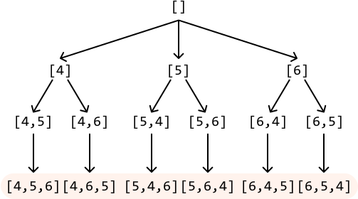
Har safar permutatsiyaga yetganda (ya'ni qurayotgan permutatsiya n o'lchamiga yetganda, bu yerda n kirish massivining uzunligini bildiradi), uni natijamizga qo'shamiz.
Holat maydoni daraxtini o'tish Barcha permutatsiyalarni yaratish holat maydoni daraxtini o'tish orqali amalga oshirilishi mumkin.
Bu daraxtdagi har bir tugun, barg tugunlardan tashqari, permutatsiya nomzodini ifodalaydi: biz qurayotgan qisman to'ldirilgan permutatsiya. Ildiz tugun bo'sh permutatsiyani ifodalaydi va daraxtga chuqurroq kirganimizda har bir permutatsiya nomzodiga element qo'shiladi. Barg tugunlar tugallangan permutatsiyalarni ifodalaydi.
Ildiz tugundan boshlab, bu daraxtni backtracking yordamida o'tishimiz mumkin:
- Ishlatilmagan son tanlang va uni joriy permutatsiya nomzodiga qo'shing. Ushbu sonni used hash set ga qo'shib, u ishlatilgan deb belgilang.
- Uning tarmoqlarini o'rganish uchun ushbu yangilangan permutatsiya nomzodi bilan rekursiv chaqiruv qiling.
- Backtrack qiling: joriy nomzod massiviga va used hash set ga qo'shgan oxirgi sonni olib tashlang.
Permutatsiya nomzodi n uzunligiga yetganda, uni natijamizga qo'shamiz.
Amalga Oshirish
from typing import List, Set

def find_all_permutations(nums: List[int]) -> List[List[int]]:
    res = []
    backtrack(nums, [], set(), res)
    return res

def backtrack(nums: List[int], candidate: List[int], used: Set[int], res: List[List[int]]) -> None:
    # If the current candidate is a complete permutation, add it to the result.
    if len(candidate) == len(nums):
        res.append(candidate[:])
        return
    for num in nums:
        if num not in used:
            # Add 'num' to the current permutation and mark it as used.
            candidate.append(num)
            used.add(num)
            # Recursively explore all branches using the updated permutation
            # candidate.
            backtrack(nums, candidate, used, res)
            # Backtrack by reversing the changes made.
            candidate.pop()
            used.remove(num)
Murakkablik Tahlili
Vaqt murakkabligi: find_all_permutations ning vaqt murakkabligi O(n * n!). Ildizdan boshlab, rekursiv ravishda n nomzodni o'rganamiz. Bu n nomzodlarning har biri uchun yana n-1 nomzodlarni, keyin n-2 ni va hokazo o'rganamiz. n! permutatsiyalarning har biri uchun uning nusxasini olib natijaga qo'shamiz, bu O(n) vaqt oladi.
Xotira murakkabligi: Rekursiya daraxtining maksimal chuqurligi n bo'lgani uchun O(n). Algoritm shuningdek candidate va used ma'lumotlar strukturalarini saqlaydi, ikkalasi ham O(n) xotira sarflaydi.
Barcha To'plamlarni Topish
Barcha To'plamlarni Topish
Berilgan noyob butun sonlar to'plamining barcha mumkin bo'lgan to'plamlarini qaytaring. Har bir to'plam istalgan tartibda bo'lishi mumkin va to'plamlar istalgan tartibda qaytarilishi mumkin.
Misol:
Input: nums = [4, 5, 6]
Output: [[], [4], [4, 5], [4, 5, 6], [4, 6], [5], [5, 6], [6]]
Intuitsiya
Bu masalani hal qilish uchun asosiy intuitsiya shundaki, har bir to'plam kirish massividagi har bir son uchun aniq qaror qabul qilish orqali shakllanadi: sonni kiritish yoki chiqarib tashlash. Masalan, [4, 5, 6] massividan [4, 6] to'plami 4 ni kiritish, 5 ni chiqarib tashlash va 6 ni kiritish orqali yaratiladi.
Holat maydoni daraxti [4, 5, 6] kirish massivini ko'rib chiqaylik. Daraxtning ildiz tugunidan — bo'sh to'plamdan — boshlaylik:

Bu yerdan qanday tarmoqlanishni aniqlash uchun element kiritish yoki chiqarib tashlash qarorimizni ko'rib chiqaylik. Bu qarorni kirish massivining birinchi elementi 4 bilan amalga oshiraylik:
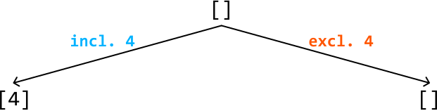
Bu to'plamlarning har biri uchun jarayonni takrorlaymiz, ikkinchi element uchun xuddi shu tanlov asosida yana tarmoqlanamiz: uni kiritish yoki chiqarib tashlash:
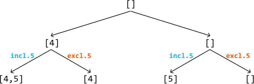
Nihoyat, uchinchi element uchun ushbu elementni kiritish yoki chiqarib tashlashga qarab har bir mavjud to'plam uchun tarmoqlanishni davom ettiramiz:
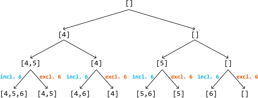
Ushbu holat maydoni daraxtida muhim nars yetishmaydi: daraxtning har bir tugunida kirish massivining qaysi elementiga qaror qabul qilayotganimizni bilish usuli. Buning uchun i indeksidan foydalanishimiz mumkin:
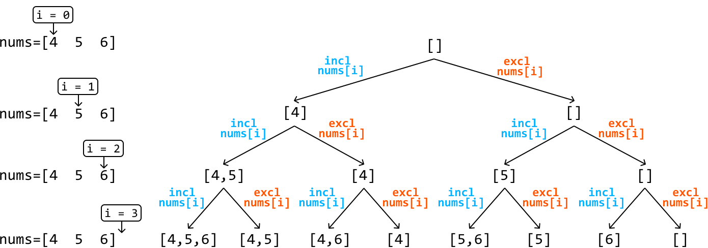
Ko'rsatilganidek, daraxtning oxirgi darajasi (ya'ni i == n bo'lganda, n kirish massivining uzunligini bildiradi) kirish massivining barcha to'plamlarini o'z ichiga oladi. Bu to'plamlarning har birini natijamizga qo'shishimiz mumkin. Ushbu to'plamlarga yetish uchun daraxtni o'tishimiz kerak, va backtracking buning uchun juda qulay.
Amalga Oshirish
from typing import List

def find_all_subsets(nums: List[int]) -> List[List[int]]:
    res = []
    backtrack(0, [], nums, res)
    return res

def backtrack(i: int, curr_subset: List[int], nums: List[int], res: List[List[int]]) -> None:
    # Base case: if all elements have been considered, add the current subset to the
    # output.
    if i == len(nums):
        res.append(curr_subset[:])
        return
    # Include the current element and recursively explore all paths that branch from
    # this subset.
    curr_subset.append(nums[i])
    backtrack(i + 1, curr_subset, nums, res)
    # Exclude the current element and recursively explore all paths that branch from
    # this subset.
    curr_subset.pop()
    backtrack(i + 1, curr_subset, nums, res)
Murakkablik Tahlili
Vaqt murakkabligi: O(2^n * n). Holat maydoni daraxti n chuqurlikka va 2 tarmoqlanish omiliga ega. Yaratilgan 2^n to'plamlarning har biri uchun nusxa olib natijaga qo'shamiz, bu O(n) vaqt oladi.
Xotira murakkabligi: Rekursiya daraxtining maksimal chuqurligi n bo'lgani uchun O(n).
N Malikalar
N Malikalar
n x n o'lchamdagi shaxmat taxtasi mavjud. Maqsadingiz — hech ikki malika bir-birini hujum qilmasligi uchun taxtaga n ta malika joylashtirish. Bu mumkin bo'lgan alohida konfiguratsiyalar sonini qaytaring.
Misol:
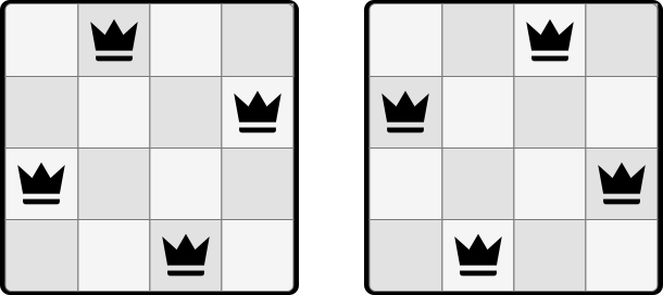
Input: n = 4
Output: 2
Intuitsiya
Malikalar vertikal, gorizontal va diagonal yo'nalishlarda harakat qila oladi:
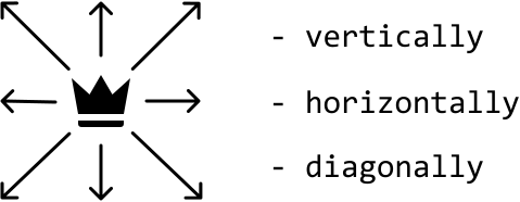
Shuning uchun taxtaning biror katagiga malika faqat quyidagi hollarda joylashtirish mumkin:
- Ushbu katagning xuddi shu satrida boshqa malika yo'q.
- Ushbu katagning xuddi shu ustunida boshqa malika yo'q.
- Ushbu katagning diagonallarida boshqa malika yo'q.
Maliklarni joylash - backtracking Oddiy strategiya — bir vaqtda taxtaga bitta malika qo'yish, har bir yangi malika hujum qilib bo'lmaydigan xavfsiz katakka joylashtirilishiga ishonch hosil qilish. Agar malika xavfsiz joylashtira olmasak, demak oldindan joylashtirilgan bir yoki bir necha malika qayta joylashtirilishi kerak.
Backtracking-ni yanada samarali qilish uchun har bir malikani yangi satrga joylashtirish mumkin. Shunday qilib, bir xil satrdagi malikalar o'rtasidagi ziddiyatlar haqida qayg'urmasdan, faqat yangi malika joylashtirilgan katagning bir xil ustuni va diagonallari bo'ylab qarama-qarshi malika borligini tekshirishimiz kerak.
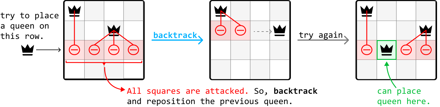
Ushbu backtracking jarayonining n = 4 uchun qisman holat maydoni daraxti quyida tasvirlangan:
Qarama-qarshi malikalarni aniqlash Bu masaladagi qiyinliklardan biri — katak boshqa malika tomonidan hujum qilinayotganini aniqlash. Buni samarali tekshirish uchun hash set-lardan foydalanishimiz mumkin.
E'tibor bering, satrlar uchun hash set kerak emas, chunki biz har doim har bir malikani boshqa satrga joylashtirамiz. Ustunlar uchun har safar (r, c) katagiga yangi malika joylashtirgan paytimizda, ushbu katagning ustun id sini (c) ustun hash set iga qo'shishimiz mumkin.
Diagonallar uchun: diagonal r - c id yordamida, anti-diagonal esa r + c id yordamida aniqlanishi mumkin.
Bu yerda asosiy kuzatuv shundaki, istalgan (r, c) katak uchun uning diagonali r - c id yordamida, anti-diagonali esa r + c id yordamida aniqlanishi mumkin.
Malika joylashtirish va olib tashlash Endi qarama-qarshi malikalarni aniqlash usuli borligini bilib, «malika joylashtirish» amali uning ustun, diagonal va anti-diagonal id larini mos hash set larga qo'shishni anglatishini bilamiz. Aksincha, malikani olib tashlash uchun ushbu id larni hash set lardan olib tashlaymiz.
Amalga Oshirish
from typing import Set

res = 0

def n_queens(n: int) -> int:
   dfs(0, set(), set(), set(), n)
   return res

def dfs(r: int, diagonals_set: Set[int], anti_diagonals_set: Set[int], cols_set: Set[int], n: int) -> None:
    global res
    # Termination condition: If we have reached the end of the rows, we've placed all
    # 'n' queens.
    if r == n:
        res += 1
        return
    for c in range(n):
        curr_diagonal = r - c
        curr_anti_diagonal = r + c
        # If there are queens on the current column, diagonal or anti-diagonal, skip
        # this square.
        if (c in cols_set or curr_diagonal in diagonals_set or curr_anti_diagonal in anti_diagonals_set):
            continue
        # Place the queen by marking the current column, diagonal, and anti-diagonal
        # as occupied.
        cols_set.add(c)
        diagonals_set.add(curr_diagonal)
        anti_diagonals_set.add(curr_anti_diagonal)
        # Recursively move to the next row to continue placing queens.
        dfs(r + 1, diagonals_set, anti_diagonals_set, cols_set, n)
        # Backtrack by removing the queen's marks.
        cols_set.remove(c)
        diagonals_set.remove(curr_diagonal)
        anti_diagonals_set.remove(curr_anti_diagonal)
Murakkablik Tahlili
Vaqt murakkabligi: O(n!). Birinchi malika uchun n ta tanlov mavjud. Ikkinchi malika uchun n-a ta tanlov bor, bu yerda a birinchi malika tomonidan ikkinchi satrdagi hujum qilinadigan kataklar sonini bildiradi. Bu tendentsiya taxminan qidiruv maydonining faktorial o'sishiga olib keladi.
Xotira murakkabligi: Rekursiya daraxtining maksimal chuqurligi n bo'lgani uchun O(n). Hash set lar ham ushbu xotira murakkabligiga hissa qo'shadi, chunki ularning har biri n tagacha qiymat saqlaydi.
Yig'indining Kombinatsiyalari
Yig'indining Kombinatsiyalari
Butun sonlar massivi va maqsad qiymat berilgan. Har bir kombinatsiyadagi sonlarning yig'indisi maqsadga teng bo'lgan massivdagi barcha noyob kombinatsiyalarni toping. Massivdagi har bir son kombinatsiyada cheklanmagan marta ishlatilishi mumkin.
Misol:
Input: nums = [1, 2, 3], target = 4
Output: [[1, 1, 1, 1], [1, 1, 2], [1, 3], [2, 2]]
Cheklovlar:
- nums dagi barcha butun sonlar musbat va noyob.
- Maqsad qiymat musbat.
- Natija takroriy kombinatsiyalarni o'z ichiga olmasligi kerak. Masalan, [1, 1, 2] va [1, 2, 1] bir xil kombinatsiya hisoblanadi.
Intuitsiya
Kirish massividagi har bir butun sonni xohlagan marta ishlatishimiz mumkin bo'lgani uchun, cheksiz sonli kombinatsiyalar yaratishimiz mumkin. Buni boshqarish uchun qidiruvimizni toraytishimiz kerak.
Bu borada yordam beradigan muhim nuqta shundaki, butun sonlar massividagi barcha qiymatlar musbat butun sonlardir. Bu kombinatsiyaga ko'proq qiymatlar qo'shganimiz sari uning yig'indisi ortishini anglatadi. Shuning uchun kombinatsiya yig'indisi maqsad qiymatiga teng yoki undan oshib ketishi bilanoq kombinatsiya qurishni to'xtatishimiz kerak.
Takrorlarning oldini olish uchun universal ifodalashni ta'minlash uchun kombinatsiyalardagi butun sonlar asl massivdagi kabi tartibda paydo bo'lishini ta'minlashimiz mumkin. Buni amalga oshirish uchun start_index dan foydalanamiz.
Holat maydoni daraxti [1, 2, 3] kirish massivi va 4 maqsadini ko'rib chiqaylik.

Bu yondashuv bilan bog'liq bir muammo shundaki, takroriy kombinatsiyalar paydo bo'ladi. Bu takrorlarning oldini olish uchun start_index dan foydalanamiz:
Dastlab, ildiz kombinatsiyasi uchun start_index 0 ga o'rnatiladi. Har bir kombinatsiyani rekursiv ravishda qurar ekanmiz, start_index qo'shilayotgan joriy elementning indeksiga yangilanadi.
Amalga Oshirish
Maqsad qiymatimizni qayta maqsadga muvofiq ishlatamiz — kombinatsiyaga son qo'shish uchun tanlaganda, maqsad qiymatini o'sha songa kamaytiramiz. 0 maqsadiga yetganda, to'g'ri kombinatsiya topilgan. Agar maqsad manfiy bo'lib qolsa, joriy tarmoqni tugatamiz.
from typing import List

def combinations_of_sum_k(nums: List[int], target: int) -> List[List[int]]:
    res = []
    dfs([], 0, nums, target, res)
    return res

def dfs(combination: List[int], start_index: int, nums: List[int], target: int,
        res: List[List[int]]) -> None:
    # Termination condition: If the target is equal to 0, we found a combination
    # that sums to 'k'.
    if target == 0:
        res.append(combination[:])
        return
    # Termination condition: If the target is less than 0, no more valid
    # combinations can be created.
    if target < 0:
        return
    # Starting from start_index, explore all combinations after adding nums[i].
    for i in range(start_index, len(nums)):
        # Add the current number to create a new combination.
        combination.append(nums[i])
        # Recursively explore all paths that branch from this new combination.
        dfs(combination, i, nums, target - nums[i], res)
        # Backtrack.
        combination.pop()
Murakkablik Tahlili
Vaqt murakkabligi: O(n^(target/m)), bu yerda n massiv uzunligini, m esa eng kichik nomzodni bildiradi. Rekursiya daraxti eng kichik nomzodlarning yig'indisi maqsadga yetguncha yoki undan oshib ketguncha tarmoqlanadi, natijada target/m chuqurlikdagi daraxt hosil bo'ladi.
Xotira murakkabligi: O(target/m), bu rekursiv chaqiruv steki chuqurligi va kombinatsiya ro'yxatini o'z ichiga oladi.
Telefon Klaviaturasi Kombinatsiyalari
Telefon Klaviaturasi Kombinatsiyalari
Sizga 2 dan 9 gacha bo'lgan raqamlarni o'z ichiga olgan satr berilgan. Har bir raqam an'anaviy telefon klaviaturasidagi harflar to'plamiga mos keladi:
| 1 | 2 abc | 3 def |
| 4 ghi | 5 jkl | 6 mno |
| 7 pqrs | 8 tuv | 9 wxyz |
Kirish raqamlari ifodalashi mumkin bo'lgan barcha mumkin bo'lgan harf kombinatsiyalarini qaytaring.
Misol:
Input: digits = '69'
Output: ['mw', 'mx', 'my', 'mz', 'nw', 'nx', 'ny', 'nz', 'ow', 'ox', 'oy', 'oz']
Intuitsiya
Satrdagi har bir raqamda qaror qabul qilishimiz kerak: bu raqam qaysi harfni ifodalaydi?
Holat maydoni daraxti "69" kirish satrini ko'rib chiqaylik. Daraxtning ildiz tugunidan — bo'sh satrdan — boshlaylik:

Birinchi raqam 6 da kombinatsiyamizni 'm', 'n' yoki 'o' bilan boshlash tanlovimiz bor:

Yaratgan bu kombinatsiyalarning har biri uchun yangi qaror qabul qilishimiz kerak: 9-raqamning qaysi harfini ('w', 'x', 'y', 'z') tanlaymiz?
Ushbu holat maydoni daraxtida muhim nars yetishmaydi — har bir tugunning qaysi raqam bo'yicha qaror qabul qilayotganligi haqida ma'lumot. Har bir tugunning qaysi raqamni ko'rib chiqayotganligini aniqlash uchun i indeksidan foydalanishimiz mumkin:
Raqamlarni harflarga moslashtirish Nihoyat, qaysi harflar qaysi raqamlarga mos kelishini aniqlash usulini topishimiz kerak. Bu maqsad uchun hash map juda qulay.
Amalga Oshirish
def phone_keypad_combinations(digits: str) -> List[str]:
    keypad_map = {
        '2': 'abc', '3': 'def', '4': 'ghi', '5': 'jkl',
        '6': 'mno', '7': 'pqrs', '8': 'tuv', '9': 'wxyz'
    }
    res = []
    backtrack(0, [], digits, keypad_map, res)
    return res

def backtrack(i: int, curr_combination: List[str], digits: str,
             keypad_map: Dict[str, str], res: List[str]) -> None:
    # Termination condition: if all digits have been considered, add the
    # current combination to the output list.
    if len(curr_combination) == len(digits):
        res.append("".join(curr_combination))
        return
    for letter in keypad_map[digits[i]]:
       # Add the current letter.
        curr_combination.append(letter)
        # Recursively explore all paths that branch from this combination.
        backtrack(i + 1, curr_combination, digits, keypad_map, res)
        # Backtrack by removing the letter we just added.
        curr_combination.pop()
Murakkablik Tahlili
Vaqt murakkabligi: O(n * 4^n). Holat maydoni daraxti barcha n element uchun qaror qabul qilinguncha, 4 gacha tarmoqlanish omili bilan tarmoqlanadi. Yaratilgan 4^n kombinatsiyalarning har biri uchun uni satrga aylantirib natija ro'yxatiga qo'shamiz, bu O(n) vaqt oladi.
Xotira murakkabligi: Rekursiv chaqiruv steki tufayli O(n), bu n ning maksimal chuqurligigacha o'sishi mumkin.
Suhbat Maslahat
Maslahat: Ahamiyatsiz amalga oshirishlarni o'tkazib yuborishingiz mumkinligini tekshiring.
Suhbat davomida vaqtni samarali boshqarish juda muhim. Agar ushbu masaladagi keypad_map ni yaratish kabi ahamiyatsiz va ko'p vaqt talab qiladigan vazifaga duch kelsangiz, suhbatdosh uni o'tkazib yuborishga yoki suhbatda vaqt qolsa keyinroq amalga oshirishga ruxsat berishi mumkin.
Dinamik Dasturlash
Dinamik Dasturlashga Kirish
Dinamik Dasturlashga Kirish
Dinamik dasturlash (DP) birinchi qarashda murakkab tuyulishi mumkin, lekin biz uni boshqariladigan kontseptlar va texnikalarga bo'lamiz. Avval DP ning kattaroq maqsadini tushunish uchun uning umumiy manzarasini ko'rib chiqaylik.
Ba'zi masalalar kichik masalalarga bo'linishi mumkin, bu yerda har bir kichik masala asosiy masalaning kichik versiyasidir. Bu kichik masalalar o'zlari ham ko'proq kichik masalalarga bo'linishi mumkin. Rekursiya ko'pincha bunday masalalarni hal qilish uchun ishlatiladi, bu yerda har bir kichik masalani hal qilish uchun rekursiv chaqiruvlar amalga oshiriladi.
Biroq, rekursiv jarayonda bir xil kichik masalani bir necha marta yaratish va hal qilish mumkin, bu esa keraksiz xarajatlarga olib kelishi mumkin.
DP buning yechimi. Bu har bir kichik masalaning yechimlarini saqlash texnikasidan iborat bo'lib, ularga qayta ehtiyoj tug'ilganda foydalanish imkonini beradi. Boshqacha aytganda, bu har bir kichik masala ko'pi bilan bir marta hal qilinishini ta'minlovchi samarali vosita.
- Optimal kichik tuzilma: masalaning optimal yechimi uning kichik masalalarining optimal yechimlaridan tuzilishi mumkin.
- Qoplanadigan kichik masalalar: masalani hal qilish jarayonida bir xil kichik masalalar bir necha marta hal qilinsa.
- Takrorlanish munosabati: masala yechimini uning kichik masalalarining yechimlari orqali ifodalaydigan formula.
- Asosiy holatlar: masalaning eng oddiy holatlari, bu yerda yechim allaqachon ma'lum va uni ko'proq kichik masalalarga bo'lish shart emas.
Birinchi ikkita atama masalaning DP yordamida hal qilinishi uchun zarur bo'lgan muhim xususiyatlar. Oxirgi ikkita atama esa har bir DP yechimining muhim tarkibiy qismlari.
Hayotiy Misol
So'z segmentatsiyasi: Qidiruv tizimlari DP ni «so'z segmentatsiyasi» deb ataladigan jarayonda qo'llaydi. Foydalanuvchilar bo'sh joysiz qidiruv so'rovi kiritsalar, DP to'g'ri so'zlarni tashkil etish uchun bo'shliqlar qo'shilishi mumkinligini aniqlash uchun qo'llaniladi.
Bob Rejasi
Ushbu bobdagi har bir DP masalasining tabiati juda noyob, lekin soddalik uchun ularni ikki toifaga ajratdik: bir o'lchamli DP (1D-DP) va ikki o'lchamli DP (2D-DP).
Zinapoyaga Ko'tarilish
Zinapoyaga Ko'tarilish
Har safar 1 yoki 2 qadam olish orqali n qadamli zinapoyaga ko'tarilishning alohida usullar sonini aniqlang.
Misol:
Input: n = 4
Output: 5
Intuitsiya - Yuqoridan Pastga
Kuch bilan yechim — 1 yoki 2 qadam olishning barcha mumkin bo'lgan kombinatsiyalarini ko'rib chiqish. i-qadamga yetish uchun u i-1 yoki i-2 qadamdan yetib kelinishi kerak.
climbing_stairs(n) = climbing_stairs(n - 1) + climbing_stairs(n - 2)
Asosiy holatlar: n 1 ga teng bo'lsa, 1 ni qaytaring. n 2 ga teng bo'lsa, 2 ni qaytaring.
Bu yechim yuqoridan pastga yechim hisoblanadi, chunki u asosiy masaladan boshlab rekursiv ravishda kichik kichik masalalarga bo'linadi.
Rekursiya daraxtida bir xil kichik masalani bir necha marta (masalan, climbing_stairs(4) ikki marta) chaqirish orqali takroriy ish bajarishimizni payqagan bo'lsangiz kerak. Bu qoplanadigan kichik masalalarni ko'rsatadi. Aynan shu yerda memoizatsiya ishga kiradi.
Doimiy vaqtda kirish uchun kichik masalalar natijalarini saqlash maqsadida memoizatsiya uchun hash map ishlatamiz.
Amalga Oshirish - Yuqoridan Pastga
memo = {}

def climbing_stairs_top_down(n: int) -> int:
    if n <= 2:
        return n
    if n in memo:
        return memo[n]
    memo[n] = climbing_stairs_top_down(n - 1) + climbing_stairs_top_down(n - 2)
    return memo[n]
Murakkablik Tahlili
Vaqt murakkabligi: Memoizatsiyasiz O(2^n). Memoizatsiya bilan O(n). Xotira murakkabligi: Rekursiv chaqiruv steki va memoizatsiya massivi tufayli O(n).
Intuitsiya - Pastdan Yuqoriga
Odatda, yuqoridan pastga memoizatsiya yordamida hal qilinishi mumkin bo'lgan har qanday masala memoizatsiya massivini DP massiviga o'tkazish orqali pastdan yuqoriga DP yondashuvi bilan ham hal qilinishi mumkin.
dp[n] = dp[n - 1] + dp[n - 2]
Asosiy holatlar: dp[1] = 1, dp[2] = 2. dp[n] ni qaytaring.
Amalga Oshirish - Pastdan Yuqoriga
def climbing_stairs_bottom_up(n: int) -> int:
    if n <= 2:
        return n
    dp = [0] * (n + 1)
    dp[1], dp[2] = 1, 2
    for i in range(3, n + 1):
        dp[i] = dp[i - 1] + dp[i - 2]
    return dp[n]
Optimallashtirish - Pastdan Yuqoriga
DP massivining faqat oldingi ikki qiymatiga kirishimiz kerak. one_step_before va two_steps_before nomli ikki o'zgaruvchidan foydalanamiz.
def climbing_stairs_bottom_up_optimized(n: int) -> int:
    if n <= 2:
        return n
    one_step_before, two_steps_before = 2, 1
    for i in range(3, n + 1):
        current = one_step_before + two_steps_before
        two_steps_before = one_step_before
        one_step_before = current
    return one_step_before
Suhbat Maslahat
Agar pastdan yuqoriga yechimni topishda qiynalsangiz, yuqoridan pastga yechimdan boshlashga urining. Avval yuqoridan pastga yechim loyihalash ko'pincha osonroq, chunki avval takrorlanish munosabatini aniqlashimiz, keyin esa uni optimallashtirish uchun memoizatsiya qo'llashimiz mumkin.
Minimal Tanga Kombinatsiyasi
Minimal Tanga Kombinatsiyasi
Sizga tanga qiymatlari massivi va maqsad pul miqdori berilgan. Maqsad miqdorini yig'ish uchun kerakli minimal tanga sonini qaytaring. Agar bu mumkin bo'lmasa, -1 ni qaytaring. Har bir tangadan cheksiz miqdor mavjud deb faraz qilishingiz mumkin.
-Misol:
Input: coins = [1, 2, 3], target = 5
Output: 2
Tushuntirish: 5 dollar yig'ish uchun bitta 2 dollarlik va bitta 3 dollarlik tanga ishlatamiz.
-Misol:
Input: coins = [2, 4], target = 5
Output: -1
Intuitsiya - Yuqoridan Pastga
Bu masalada ishlatishimiz mumkin bo'lgan tanga sonida cheklash yo'q, bu esa kuch bilan yechishni imkonsiz qiladi. Tanga ishlatish kamaytirilgan maqsad bilan yangi kichik masalani yaratadi.



min_coin_combination(target) = 1 + min(min_coin_combination(target - coin_i) | coin_i in coins)
Asosiy holat: maqsad 0 ga teng bo'lganda, 0 ni qaytaring. Memoizatsiya ortiqcha hisoblashlarni oldini olish uchun yechimlarni saqlaydi.
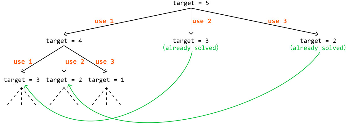
Amalga Oshirish - Yuqoridan Pastga
Murakkablik Tahlili
Vaqt: Memoizatsiyasiz O(n^(target/m)), memoizatsiya bilan O(target * n). Xotira: O(target).
Intuitsiya - Pastdan Yuqoriga
Zinapoyaga Ko'tarilish masalasidagi xuddi shu texnikadan foydalanib, yuqoridan pastga yechimimizni pastdan yuqoriga yechimga aylantiramiz.
for t in range(1, target + 1):
    for coin in coins:
        if coin <= t:
            dp[t] = min(dp[t], 1 + dp[t - coin])
Amalga Oshirish - Pastdan Yuqoriga
def min_coin_combination_bottom_up(coins, target):
    dp = [float('inf')] * (target + 1)
    dp[0] = 0
    for t in range(1, target + 1):
        for coin in coins:
            if coin <= t:
                dp[t] = min(dp[t], 1 + dp[t - coin])
    return dp[target] if dp[target] != float('inf') else -1
Murakkablik Tahlili
Vaqt: O(target * n). Xotira: O(target).
Suhbat Maslahat
Masala biror narsaning minimal yoki maksimalini so'raganda, bu DP masalasi bo'lishi mumkin. 'minimal', 'maksimal', 'eng uzun' yoki 'eng qisqa' kabi kalit so'zlar DP yondashuvini taklif qiladi.
Matritsa Yo'llari
Matritsa Yo'llari
Siz m x n matritsaning yuqori chap burchagida turibsiz va faqat pastga yoki o'ngga harakat qilishingiz mumkin. Pastki o'ng burchakka yetish uchun qancha noyob yo'l borligini aniqlang.
Misol:

Input: m = 3, n = 3
Output: 6
Intuitsiya
Istalgan katakka yo'llar soni yuqoridagi katak va chap tomondagi katakdan yo'llar yig'indisiga teng.
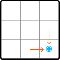
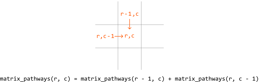
dp[r][c] = dp[r - 1][c] + dp[r][c - 1]
Asosiy holatlar: 0-satr va 0-ustundagi barcha kataklar uchun aynan bitta yo'l bor (1 ga o'rnatiladi).
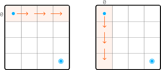
Amalga Oshirish
def matrix_pathways(m, n):
    dp = [[1] * n for _ in range(m)]
    for r in range(1, m):
        for c in range(1, n):
            dp[r][c] = dp[r - 1][c] + dp[r][c - 1]
    return dp[m - 1][n - 1]
Murakkablik Tahlili
Vaqt: O(m*n). Xotira: O(m*n).
Optimallashtirish
Faqat ikkita qator saqlash kerak: prev_row va curr_row. Xotirani O(n) ga kamaytiradi.
def matrix_pathways_optimized(m, n):
    prev_row = [1] * n
    for r in range(1, m):
        curr_row = [1] * n
        for c in range(1, n):
            curr_row[c] = prev_row[c] + curr_row[c - 1]
        prev_row = curr_row
    return prev_row[n - 1]
Mahalla O'g'irligʻi
Mahalla O'g'irligʻi
Siz har bir uyda ma'lum miqdor pul saqlanadigan ko'chada uylarni o'g'irlamoqchi siz. Mahallada ikki qo'shni uy o'g'irlanganda signalizatsiya qo'zg'atadigan xavfsizlik tizimi bor. Signalizatsiyani ishga tushirmasdan o'g'irlanishi mumkin bo'lgan maksimal pul miqdorini qaytaring.
Misol:
Input: houses = [200, 300, 200, 50]
Output: 400
Tushuntirish: 0 va 2 indeksli uylardan o'g'irlash 200 + 200 = 400 dollar beradi.
Intuitsiya
Greedy yondashuvi uzoq muddatli oqibatlarni e'tiborsiz qoldiradi. i-uyda ikki tanlovimiz bor: uni o'tkazib yuborish (foyda = dp[i-1]) yoki o'g'irlash (foyda = houses[i] + dp[i-2]).
dp[i] = max(dp[i - 1], houses[i] + dp[i - 2])
Asosiy holatlar: dp[0] = houses[0], dp[1] = max(houses[0], houses[1]).
Amalga Oshirish
def neighborhood_burglary(houses):
    if not houses: return 0
    if len(houses) == 1: return houses[0]
    dp = [0] * len(houses)
    dp[0] = houses[0]
    dp[1] = max(houses[0], houses[1])
    for i in range(2, len(houses)):
        dp[i] = max(dp[i - 1], houses[i] + dp[i - 2])
    return dp[len(houses) - 1]
Murakkablik Tahlili
Vaqt: O(n). Xotira: O(n).
Optimallashtirish
Faqat oldingi ikki qiymat kerak. prev_max_profit va prev_prev_max_profit o'zgaruvchilaridan foydalanamiz. Xotirani O(1) ga kamaytiradi.
def neighborhood_burglary_optimized(houses):
    if not houses: return 0
    if len(houses) == 1: return houses[0]
    prev_max_profit = max(houses[0], houses[1])
    prev_prev_max_profit = houses[0]
    for i in range(2, len(houses)):
        curr_max_profit = max(prev_max_profit, houses[i] + prev_prev_max_profit)
        prev_prev_max_profit = prev_max_profit
        prev_max_profit = curr_max_profit
    return prev_max_profit
Eng Uzun Umumiy Ketma-Ketlik
Eng Uzun Umumiy Ketma-Ketlik
Ikki satr berilgan. Ularning eng uzun umumiy ketma-ketligining (LCS) uzunligini toping. Ketma-ketlik — satrdan qolgan elementlar tartibini o'zgartirmasdan nol yoki undan ko'p element o'chirish orqali olingan belgilar to'plami.
Misol:
Input: s1 = 'acabac', s2 = 'aebab'
Output: 3
Intuitsiya
Ikki holat: (1) teng belgilar: ularni kiritamiz, LCS(i,j) = 1 + LCS(i+1, j+1). (2) farqli belgilar: max(s1[i] ni istisno qilgan LCS, s2[j] ni istisno qilgan LCS).
if s1[i] == s2[j]: LCS(i, j) = 1 + LCS(i + 1, j + 1)
if s1[i] != s2[j]: LCS(i, j) = max(LCS(i + 1, j), LCS(i, j + 1))
DP formulasi: dp[i][j]. Asosiy holatlar: dp[len(s1)][j] = 0 va dp[i][len(s2)] = 0. dp[0][0] ni qaytaring.
Amalga Oshirish
def longest_common_subsequence(s1, s2):
    dp = [[0] * (len(s2) + 1) for _ in range(len(s1) + 1)]
    for i in range(len(s1) - 1, -1, -1):
        for j in range(len(s2) - 1, -1, -1):
            if s1[i] == s2[j]:
                dp[i][j] = 1 + dp[i + 1][j + 1]
            else:
                dp[i][j] = max(dp[i + 1][j], dp[i][j + 1])
    return dp[0][0]
Murakkablik Tahlili
Vaqt: O(m*n). Xotira: O(m*n).
Optimallashtirish
Faqat ikkita qator kerak: curr_row va prev_row. Xotira O(n) ga kamayadi.
def longest_common_subsequence_optimized(s1, s2):
    prev_row = [0] * (len(s2) + 1)
    for i in range(len(s1) - 1, -1, -1):
        curr_row = [0] * (len(s2) + 1)
        for j in range(len(s2) - 1, -1, -1):
            if s1[i] == s2[j]:
                curr_row[j] = 1 + prev_row[j + 1]
            else:
                curr_row[j] = max(prev_row[j], curr_row[j + 1])
        prev_row = curr_row
    return prev_row[0]
Satrdagi Eng Uzun Palindrom
Satrdagi Eng Uzun Palindrom
Berilgan satr ichidagi eng uzun palindromik pastki satrni qaytaring.
Misol:
Input: s = 'abccbaba'
Output: 'abccba'
Intuitsiya
s[i:j] pastki satri palindrom bo'ladi agar: (1) s[i] == s[j] va (2) s[i+1:j-1] ham palindrom bo'lsa.
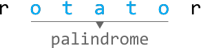
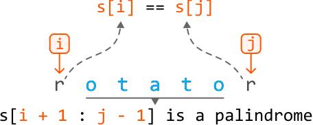
dp[i][j] = True if s[i] == s[j] and dp[i + 1][j - 1]
Asosiy holatlar: Uzunligi 1 bo'lgan barcha pastki satrlar palindrom (dp[i][i] = True). Uzunligi 2 bo'lgan pastki satrlar ikki belgi bir xil bo'lsa palindrom.
Eng uzun palindromni start_index va max_len yordamida kuzatib boring. s[start_index : start_index + max_len] ni qaytaring.
Amalga Oshirish
def longest_palindrome_in_a_string(s):
    n = len(s)
    if n == 0: return ''
    dp = [[False] * n for _ in range(n)]
    max_len = 1
    start_index = 0
    for i in range(n):
        dp[i][i] = True
    for i in range(n - 1):
        if s[i] == s[i + 1]:
            dp[i][i + 1] = True
            max_len = 2
            start_index = i
    for substring_len in range(3, n + 1):
        for i in range(n - substring_len + 1):
            j = i + substring_len - 1
            if s[i] == s[j] and dp[i + 1][j - 1]:
                dp[i][j] = True
                if substring_len > max_len:
                    max_len = substring_len
                    start_index = i
    return s[start_index : start_index + max_len]
Murakkablik Tahlili
Vaqt: O(n^2). Xotira: O(n^2).
Optimallashtirilgan Yondashuv
Har bir asosiy holat markazidan tashqariga kengaytirish. Ikki tur: bitta belgi (toq) va ikki belgi (juft) markazlar.
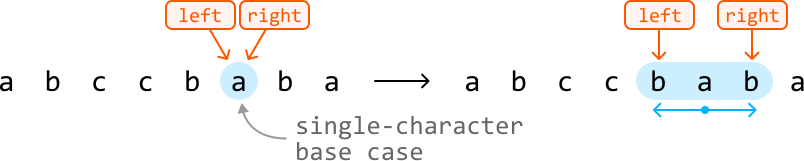
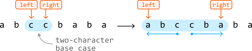
def longest_palindrome_in_a_string_expanding(s):
    n = len(s)
    start, max_len = 0, 0
    for center in range(n):
        odd_start, odd_length = expand_palindrome(center, center, s)
        if odd_length > max_len:
            start = odd_start
            max_len = odd_length
        if center < n - 1 and s[center] == s[center + 1]:
            even_start, even_length = expand_palindrome(center, center + 1, s)
            if even_length > max_len:
                start = even_start
                max_len = even_length
    return s[start : start + max_len]
Murakkablik Tahlili
Vaqt: O(n^2). Xotira: O(1).
Manacher Algoritmi
Manacher algoritmi O(n) vaqtda ishlaydi, lekin bu kodlash suhbatlarida kamdan-kam uchraydigan ixtisoslashtirilgan algoritmdir. Ko'pchilik suhbatdoshlar kuchli muammo hal qilish asoslarini ko'rsatadigan yechimlarni xohlaydi.
Maksimal Pastki Massiv Yig'indisi
Maksimal Pastki Massiv Yig'indisi
Butun sonlar massivi berilgan. Eng katta yig'indiga ega pastki massivning yig'indisini qaytaring.
Misol:
Input: nums = [3, 1, -6, 2, -1, 4, -9]
Output: 5
Tushuntirish: [2, -1, 4] pastki massivining eng katta yig'indisi 5.
Intuitsiya
Har bir son uchun max(curr_sum + num, num) ni tanlaymiz: mavjud pastki massivni davom ettirish yoki joriy elementdan yangi pastki massiv boshlash.

max_sum — eng katta curr_sum ni kuzatib boring. Bu Kadane algoritmi.
Amalga Oshirish
def maximum_subarray_sum(nums):
    if not nums: return 0
    max_sum = current_sum = float('-inf')
    for num in nums:
        current_sum = max(current_sum + num, num)
        max_sum = max(max_sum, current_sum)
    return max_sum
Murakkablik Tahlili
Vaqt: O(n). Xotira: O(1).
Intuitsiya - DP
Har bir pastki massiv ma'lum indeksda tugaydi. dp[i] = i indeksida tugaydigan maksimal pastki massiv yig'indisi.
max_subarray(i) = max(max_subarray(i - 1) + nums[i], nums[i])
dp[i] = max(dp[i - 1] + nums[i], nums[i])
Asosiy holat: dp[0] = nums[0]. Barcha dp qiymatlarining maksimalini qaytaring.
Amalga Oshirish - DP
def maximum_subarray_sum_dp(nums):
    n = len(nums)
    if n == 0: return 0
    dp = [0] * n
    dp[0] = nums[0]
    max_sum = dp[0]
    for i in range(1, n):
        dp[i] = max(dp[i - 1] + nums[i], nums[i])
        max_sum = max(max_sum, dp[i])
    return max_sum
Optimallashtirish
To'liq DP massivi o'rniga bitta o'zgaruvchidan foydalanamiz. Xotira O(1) ga kamayadi.
def maximum_subarray_sum_dp_optimized(nums):
    n = len(nums)
    if n == 0: return 0
    current_sum = nums[0]
    max_sum = nums[0]
    for i in range(1, n):
        current_sum = max(nums[i], current_sum + nums[i])
        max_sum = max(max_sum, current_sum)
    return max_sum
0/1 Knapsack
/1 Knapsack
Siz do'kon talash rejalashtirgan o'g'risan. Faqat maksimal cap birlik sig'imga ega sumkani ko'tarish mumkin. Har bir buyum (i) og'irlikka (weights[i]) va qiymatga (values[i]) ega. Olib ketishingiz mumkin bo'lgan maksimal umumiy qiymatni toping.
Misol:
Input: cap = 7, weights = [5, 3, 4, 1], values = [70, 50, 40, 10]
Output: 90
Tushuntirish: 1 va 2-buyumlarning umumiy qiymati 50 + 40 = 90 va og'irligi 3 + 4 = 7.
Intuitsiya
Har bir buyum uchun ikkilik qaror: kiritish yoki chiqarish (shuning uchun '0/1 Knapsack'). Takrorlanish munosabati:
knapsack(i, c) = max(values[i] + knapsack(i + 1, c - weights[i]), knapsack(i + 1, c))
Agar buyum sig'masa: knapsack(i, c) = knapsack(i + 1, c).
if weights[i] <= c:
    dp[i][c] = max(values[i] + dp[i + 1][c - weights[i]], dp[i + 1][c])
else:
    dp[i][c] = dp[i + 1][c]
Asosiy holatlar: barcha c uchun dp[n][c] = 0 (buyumlar yo'q), barcha i uchun dp[i][0] = 0 (sig'im yo'q). dp[0][cap] ni qaytaring.
Amalga Oshirish
def knapsack(cap, weights, values):
    n = len(values)
    dp = [[0 for x in range(cap + 1)] for x in range(n + 1)]
    for i in range(n - 1, -1, -1):
        for c in range(1, cap + 1):
            if weights[i] <= c:
                dp[i][c] = max(values[i] + dp[i + 1][c - weights[i]], dp[i + 1][c])
            else:
                dp[i][c] = dp[i + 1][c]
    return dp[0][cap]
Murakkablik Tahlili
Vaqt: O(n*cap). Xotira: O(n*cap).
Optimallashtirish
Faqat ikkita qator kerak: curr_row va prev_row. Xotira O(cap) ga kamayadi.
def knapsack_optimized(cap, weights, values):
    n = len(values)
    prev_row = [0] * (cap + 1)
    for i in range(n - 1, -1, -1):
        curr_row = [0] * (cap + 1)
        for c in range(1, cap + 1):
            if weights[i] <= c:
                curr_row[c] = max(values[i] + prev_row[c - weights[i]], prev_row[c])
            else:
                curr_row[c] = prev_row[c]
        prev_row = curr_row
    return prev_row[cap]
Matritsadagi Eng Katta Kvadrat
Matritsadagi Eng Katta Kvadrat
Ikkilik matritsadagi 1 lardan iborat eng katta kvadratning maydonini aniqlang.
Misol:
Output: 9
Intuitsiya
Kvadratlar ichida kichikroq kvadratlarni o'z ichiga oladi. (i,j) da tugaydigan kvadratning tomonlari uzunligi chap (i,j-1), yuqori (i-1,j) va yuqori-chap diagonal (i-1,j-1) da tugaydigan kvadratlarga bog'liq.
if matrix[i][j] == 1: dp[i][j] = 1 + min(dp[i - 1][j], dp[i - 1][j - 1], dp[i][j - 1])
Asosiy holatlar: 0-satr va 0-ustundagi kataklar matritsa qiymatiga (0 yoki 1) teng dp qiymatini oladi.
max_len ni kuzatib boring. Maydon uchun max_len^2 ni qaytaring.
Amalga Oshirish
def largest_square_in_a_matrix(matrix):
    if not matrix: return 0
    m, n = len(matrix), len(matrix[0])
    dp = [[0] * n for _ in range(m)]
    max_len = 0
    for j in range(n):
        if matrix[0][j] == 1:
            dp[0][j] = 1
            max_len = 1
    for i in range(m):
        if matrix[i][0] == 1:
            dp[i][0] = 1
            max_len = 1
    for i in range(1, m):
        for j in range(1, n):
            if matrix[i][j] == 1:
                dp[i][j] = 1 + min(dp[i-1][j], dp[i-1][j-1], dp[i][j-1])
                max_len = max(max_len, dp[i][j])
    return max_len ** 2
Murakkablik Tahlili
Vaqt: O(m*n). Xotira: O(m*n).
Optimallashtirish
Faqat ikkita qator kerak: prev_row va curr_row. Xotira O(m) ga kamayadi.
def largest_square_in_a_matrix_optimized(matrix):
    if not matrix: return 0
    m, n = len(matrix), len(matrix[0])
    prev_row = [0] * n
    max_len = 0
    for i in range(m):
        curr_row = [0] * n
        for j in range(n):
            if i == 0 or j == 0:
                curr_row[j] = matrix[i][j]
            else:
                if matrix[i][j] == 1:
                    curr_row[j] = 1 + min(curr_row[j-1], prev_row[j-1], prev_row[j])
            max_len = max(max_len, curr_row[j])
        prev_row, curr_row = curr_row, [0] * n
    return max_len ** 2
Greedy (Ochko'z) Algoritmlar
Greedy Algoritmlarga Kirish
Greedy Algoritmlarga Kirish
Intuitsiya
Greedy algoritmlar — har bir qaror mavjud variantlar orasida eng yaxshi darhol tanlov bo'lgan qarorlar ketma-ketligini qabul qiladigan algoritmlar sinfi.
Tasavvur qiling, A shahridan E shahriga sayohat rejalashtirmoqdasiz va yo'lda B, C va D shaharlarini ziyorat qilmoqchisiz.
Eng tez yo'lni xohlaysiz. Barcha mumkin bo'lgan yo'llarni tekshirish o'rniga, sayohatning har bir bosqichida eng qisqa vaqt talab qiladigan yo'lni tanlaysiz.
Bu amalda masalaga greedy yondashuv bo'lib, umumiy eng yaxshi yechimga erishishni maqsad qilib, har bir qadamda eng yaxshi variantni tanlaysiz.
Greedy algoritm qanday ishlaydi? Rasmiyroq aytganda, greedy algoritm greedy tanlov xususiyatiga amal qiladi, bu esa masalaning umumiy eng yaxshi yechimiga (global optimum) har bir qadamda eng yaxshi qaror qabul qilish (lokal optimum) orqali yetish mumkinligini bildiradi.
Har bir qaror faqat joriy kontekst asosida qabul qilinadi va uning kelajakdagi qadamlarga ta'sirini e'tiborsiz qoldiradi. Bu jarayon algoritm yakuniy yechimga yetguncha davom etadi.
Masalani greedy yondashuv bilan hal qilish mumkinligini qanday aniqlash Greedy yondashuvlar DP ga o'xshab, odatda optimallashtirish masalalari uchun ishlatiladi. Masalaning optimal kichik tuzilmaga ega ekanligini tekshiramiz. DP va greedy o'rtasidagi asosiy farq: greedy tanlov xususiyatiga amal qiladi, DP esa barcha mumkin bo'lgan yechimlarni ko'rib chiqadi. Barcha greedy masalalar DP yordamida hal qilinishi mumkin, lekin barcha DP masalalar greedy tarzda hal qilinmaydi.
Hayotiy Misol
Ma'lumotlarni siqishda Huffman kodlash: Huffman kodlash kirish belgilariga ularning chastotasi asosida o'zgaruvchan uzunlikdagi kodlar beradi. Greedy yondashuv doimo avval ikki eng kam chastotali belgilarni birlashtiradi, bu har bir qadamda umumiy kodlash hajmini kamaytiradi. ZIP, JPEG da qo'llaniladi.
Bob Rejasi
Greedy masalalarni hal qilish uchun universal doira taqdim etish amaliy emas, chunki ularning har biri noyob. Ushbu bob greedy tanlov xususiyati yechimga olib keladigan turli noyob holatlarni o'rganadi.
Oxiriga Sakrash
Oxiriga Sakrash
Sizga dastlab 0 indeksida joylashgan butun sonlar massivi berilgan. Har bir son joriy indeksdan maksimal sakrash masofasini ifodalaydi. Massivning oxiriga yetish mumkin yoki yo'qligini aniqlang.
-Misol:
![Jump path in [3,2,0,2,5]](https://bytebytego.com/images/courses/coding-patterns/greedy/jump-to-the-end/jump-to-the-end1-SUME32HH.svg)
Input: nums = [3, 2, 0, 2, 5]
Output: True
-Misol:
![Dead end in [2,1,0,3]](https://bytebytego.com/images/courses/coding-patterns/greedy/jump-to-the-end/jump-to-the-end2-BNR76P5W.svg)
Input: nums = [2, 1, 0, 3]
Output: False
Intuitsiya
i indeksidan yetishilishi mumkin bo'lgan eng uzoq indeks i + nums[i]. Qiyinlik 0 lardan (o'lik cho'qqilar) kelib chiqadi. Orqaga qarab fikrlang: maqsadni oxirgi indeksga o'rnating va orqaga qarab o'ting. Agar i + nums[i] >= maqsad bo'lsa, maqsad = i qiling.
Agar i + nums[i] >= maqsad bo'lsa, i indeksidan maqsadga sakrash mumkin.
Greedy tanlov: o'ngdan birinchi to'g'ri indeks yangi maqsad bo'ladi. Asl maqsadga yeta oladigan boshqa barcha indekslar ham ushbu birinchi to'g'ri indeksga yeta oladi. maqsad == 0 bo'lganda true qaytaring.
Amalga Oshirish
def jump_to_the_end(nums):
    destination = len(nums) - 1
    for i in range(len(nums) - 1, -1, -1):
        if i + nums[i] >= destination:
            destination = i
    return destination == 0
Murakkablik Tahlili
Vaqt: O(n). Xotira: O(1).
Benzin Stantsiyalari
Benzin Stantsiyalari
Benzin stantsiyalari joylashgan dumaloq yo'l mavjud. Har bir stantsiyada mashinangizni gas[i] miqdorda benzin bilan to'ldirish mumkin, va keyingi stantsiyaga o'tish cost[i] sarflaydi. Benzin tugamasdan davrani yakunlash uchun boshlash kerak bo'lgan benzin stantsiyasining indeksini toping. Agar imkonsiz bo'lsa, -1 ni qaytaring. Faqat bitta yechim mavjud deb faraz qiling.
Misol:
Input: gas = [2, 5, 1, 3], cost = [3, 2, 1, 4]
Output: 1
Intuitsiya
1-holat: sum(gas) < sum(cost) — imkonsiz, -1 qaytaring. 2-holat: sum(gas) >= sum(cost) — to'g'ri boshlash nuqtasi mavjud bo'lishi kerak.
Har bir stantsiyada sof benzindan (gas[i] - cost[i]) foydalaning. Oldinga o'tib, bak to'planadi. Agar i-stantsiyada bak < 0 bo'lsa, joriy boshlanish nuqtasidan yoki boshlanish va i o'rtasidagi biror stantsiyadan boshlash mumkin emas. start = i+1, tank = 0 ni qayta o'rnating.
Agar a stantsiyasidan b stantsiyasiga yeta olmasak, a va b o'rtasida benzin tugamasdan hech qayerdan boshlab bo'lmaydi.

Isboti: agar sum(gas) >= sum(cost) bo'lsa, ushbu greedy jarayon tomonidan topilgan to'g'ri boshlash davrani yakunlashni kafolatlaydi.
Amalga Oshirish
def gas_stations(gas, cost):
if sum(gas) < sum(cost):
return -1
start = tank = 0
for i in range(len(gas)):
tank += gas[i] - cost[i]
if tank < 0:
start, tank = i + 1, 0
return start
Murakkablik Tahlili
Vaqt: O(n). Xotira: O(1).
Suhbat Maslahat
Maslahat: Agar greedy yechimingizni rasmiy isbotlash qiyin bo'lsa, misollar bilan ko'rsating. Turli xil misollar bilan to'g'riligini ko'rsatish suhbat sharoitida yaxshi murosaga kelish hisoblanadi.
Konfetlar
Konfetlar
Siz qatorda o'tirgan, har biri ishlash reytingiga ega bolalar sinfini o'qitasiz. Qoidalar: (1) Har bir bola kamida bitta konfet olishi kerak. (2) Agar ikki qo'shni bolaning reytingi farqli bo'lsa, yuqori reytingga ega bola ko'proq konfet olishi kerak. Minimal konfetlar sonini toping.
-Misol:
Input: ratings = [4, 3, 2, 4, 5, 1]
Output: 12
Tushuntirish: Konfetlarni [3, 2, 1, 2, 3, 1] sifatida taqsimlang.
-Misol:
Input: ratings = [1, 3, 3]
Output: 4
Intuitsiya
Ikki o'tishli greedy: Birinchi o'tish (chapdan o'ngga): agar ratings[i] > ratings[i-1] bo'lsa, candies[i] = candies[i-1] + 1 qiling. Ikkinchi o'tish (o'ngdan chapga): agar ratings[i] > ratings[i+1] bo'lsa, candies[i] = max(candies[i], candies[i+1] + 1) qiling. Har bir boladan 1 konfet bilan boshlang.


Bu greedy yechim: har bir bola uchun faqat bevosita qo'shnilarini hisobga olgan holda lokal optimal tanlov. Ikki o'tish birgalikda chap va o'ng qo'shni cheklovlarining ikkalasi ham qondirilishini ta'minlaydi.
Amalga Oshirish
def candies(ratings):
n = len(ratings)
candies = [1] * n
for i in range(1, n):
if ratings[i] > ratings[i - 1]:
candies[i] = candies[i - 1] + 1
for i in range(n - 2, -1, -1):
if ratings[i] > ratings[i + 1]:
candies[i] = max(candies[i], candies[i + 1] + 1)
return sum(candies)
Murakkablik Tahlili
Vaqt: O(n). Xotira: O(n).
Saralash va Qidirish
Saralash va Qidirishga Kirish
Saralash va Qidirishga Kirish
Saralash va qidirish informatikadagi eng fundamental operatsiyalardan ikkitasi. Ushbu bobda ma'lumotlarni samarali saralash va qidirish naqsh va texnikalarini o'rganamiz.
Saralash
Saralash elementlarni ma'lum tartibda (odatda o'sish yoki kamayish tartibida) joylashtirish. Umumiy saralash algoritmlari:
- Merge Sort: O(n log n) vaqt, O(n) xotira — barqaror, bo'l va zabt et
- Quick Sort: O(n log n) o'rtacha vaqt, O(log n) xotira — joyida, bo'l va zabt et
- Counting Sort: O(n + k) vaqt, O(k) xotira — ma'lum diapazonidagi butun sonlar uchun
Qidirish
Qidirish ma'lumotlar strukturasida aniq element yoki qiymatni topish. Binary Search saralangan ma'lumotlarda qidirish uchun eng samarali algoritm:
- Binary Search: O(log n) vaqt — faqat saralangan massivlarda ishlaydi
- Chiziqli qidirish: O(n) vaqt — saralanmagan massivlarda ishlaydi
Masalalar
Ushbu bobda quyidagi masalalarni hal qilamiz:
- Bog'liq Ro'yxatni Saralash
- Massivni Saralash
- K-chi Eng Katta Butun Son
- Gollandiya Milliy Bayrog'i
Bog'liq Ro'yxatni Saralash
Bog'liq Ro'yxatni Saralash
Yakka bog'liq ro'yxatning boshi (head) berilgan. Uni o'sish tartibida saraling va saralangan ro'yxatning boshini qaytaring.
Misol:
Input: head = [4, 2, 1, 3]
Output: [1, 2, 3, 4]
Intuitsiya
Bog'liq ro'yxatni saralash uchun merge sort dan foydalanishimiz mumkin, bu bog'liq ro'yxatlarga juda mos, chunki tasodifiy kirish talab qilmaydi (quicksort dan farqli). Algoritm quyidagicha ishlaydi:
- Sekin va tez ko'rsatkich texnikasi yordamida ro'yxatni ikkiga bo'lish.
- Har bir yarmni rekursiv ravishda saralash.
- Ikki saralangan yarmni birlashtirish.
Amalga Oshirish
class ListNode:
def __init__(self, val=0, next=None):
self.val = val
self.next = next
def sort_linked_list(head: ListNode) -> ListNode:
if not head or not head.next:
return head
# Split the list into two halves
left, right = split_list(head)
# Recursively sort each half
left = sort_linked_list(left)
right = sort_linked_list(right)
# Merge the two sorted halves
return merge(left, right)
def split_list(head: ListNode):
slow, fast = head, head.next
while fast and fast.next:
slow = slow.next
fast = fast.next.next
right = slow.next
slow.next = None
return head, right
def merge(left: ListNode, right: ListNode) -> ListNode:
dummy = ListNode(0)
curr = dummy
while left and right:
if left.val <= right.val:
curr.next = left
left = left.next
else:
curr.next = right
right = right.next
curr = curr.next
curr.next = left if left else right
return dummy.next
Murakkablik Tahlili
Vaqt murakkabligi: O(n log n) — har bir bo'linish O(n), rekursiyaning O(log n) darajasi mavjud.
Xotira murakkabligi: O(log n) — rekursiv chaqiruv steki uchun.
Massivni Saralash
Massivni Saralash
Butun sonlar massivi nums berilgan. Massivni o'sish tartibida saraling va qaytaring. Masalani ichki funksiyalardan foydalanmasdan O(nlog(n)) vaqt murakkabligi va minimal xotira murakkabligi bilan hal qilishingiz kerak.
Misol:
Input: nums = [5, 2, 3, 1]
Output: [1, 2, 3, 5]
Intuitsiya
O(n log n) o'rtacha vaqt murakkabligi va O(log n) xotira murakkabligiga ega quicksort dan foydalanishimiz mumkin. Quicksort quyidagicha ishlaydi:
- Massivdan kalit (pivot) element tanlash.
- Qolgan elementlarni ikki guruhga bo'lish: kalit dan kichik elementlar va kalit dan katta elementlar.
- Ikkala guruhga xuddi shu mantiqni rekursiv qo'llash.
Shu bilan birga, elementlar diapazoni cheklangan bo'lganda counting sort dan ham foydalanish mumkin, bu k kirish qiymatlarining diapazoni bo'lgan O(n + k) vaqt murakkabligiga ega.
Amalga Oshirish
from typing import List
import random
def sort_array(nums: List[int]) -> List[int]:
quicksort(nums, 0, len(nums) - 1)
return nums
def quicksort(nums: List[int], low: int, high: int) -> None:
if low < high:
pivot_idx = partition(nums, low, high)
quicksort(nums, low, pivot_idx - 1)
quicksort(nums, pivot_idx + 1, high)
def partition(nums: List[int], low: int, high: int) -> int:
# Randomly select a pivot to avoid worst case
rand_idx = random.randint(low, high)
nums[rand_idx], nums[high] = nums[high], nums[rand_idx]
pivot = nums[high]
i = low - 1
for j in range(low, high):
if nums[j] <= pivot:
i += 1
nums[i], nums[j] = nums[j], nums[i]
nums[i + 1], nums[high] = nums[high], nums[i + 1]
return i + 1
Murakkablik Tahlili
Vaqt murakkabligi: O(n log n) o'rtacha — tasodifiy kalit tanlash bilan kamdan-kam O(n²) eng yomon holat.
Xotira murakkabligi: O(log n) — rekursiv chaqiruv steki uchun.
K-chi Eng Katta Butun Son
K-chi Eng Katta Butun Son
Saralanmagan butun sonlar massivi nums va k butun soni berilgan. Massivdagi k-chi eng katta elementni qaytaring.
Misol:
Input: nums = [3, 2, 1, 5, 6, 4], k = 2
Output: 5
Intuitsiya
Bu masalani hal qilishning ikki samarali yondashuvi mavjud:
-Yondashuv: Min-Heap
k o'lchamli min-heap ni saqlashimiz mumkin. Har bir element uchun, agar u heap ning minimumidan katta bo'lsa, minimumni ushbu element bilan almashtiramiz. Barcha elementlar qayta ishlangandan so'ng, heap ning minimumi k-chi eng katta element hisoblanadi.
Bu yondashuv O(n log k) vaqt murakkabligi va O(k) xotira murakkabligiga ega.
-Yondashuv: Quickselect
Quickselect — saralanmagan ro'yxatda k-chi kichik (yoki katta) elementni topadigan tanlov algoritmi. U quicksort ning bo'lish qadamiga asoslangan.
Bu yondashuv O(n) o'rtacha vaqt murakkabligi va O(log n) xotira murakkabligiga ega.
Amalga Oshirish
import heapq
from typing import List
def kth_largest(nums: List[int], k: int) -> int:
min_heap = []
for num in nums:
heapq.heappush(min_heap, num)
if len(min_heap) > k:
heapq.heappop(min_heap)
return min_heap[0]
import random
from typing import List
def kth_largest_quickselect(nums: List[int], k: int) -> int:
target = len(nums) - k # kth largest = (n-k)th smallest
def quickselect(low: int, high: int) -> int:
pivot_idx = random.randint(low, high)
nums[pivot_idx], nums[high] = nums[high], nums[pivot_idx]
pivot = nums[high]
i = low
for j in range(low, high):
if nums[j] <= pivot:
nums[i], nums[j] = nums[j], nums[i]
i += 1
nums[i], nums[high] = nums[high], nums[i]
if i == target:
return nums[i]
elif i < target:
return quickselect(i + 1, high)
else:
return quickselect(low, i - 1)
return quickselect(0, len(nums) - 1)
Murakkablik Tahlili
Min-Heap: Vaqt murakkabligi O(n log k), Xotira murakkabligi O(k).
Quickselect: Vaqt murakkabligi O(n) o'rtacha, O(n²) eng yomon holat, Xotira murakkabligi O(log n).
Gollandiya Milliy Bayrog'i
Gollandiya Milliy Bayrog'i
Mos ravishda qizil, oq va ko'k ranglarni ifodalovchi 0, 1 va 2 lardan iborat massiv berilgan. Massivni joyida shu tarzda saraling: avval barcha qizillar (0 lar), keyin oqlar (1 lar) va nihoyat ko'klar (2 lar) — Gollandiya milliy bayrog'i kabi.
Misol:
Input: nums = [0, 1, 2, 0, 1, 2, 0]
Output: [0, 0, 0, 1, 1, 2, 2]
Intuitsiya
Bu masala aslida uchta sonni o'sish tartibida saralashni so'raydi. Oddiy yechim — ichki saralash funksiyasidan foydalanish. Biroq, bu O(nlog(n)) yondashuv bo'lib, n massiv uzunligini bildiradi. Ammo bu muhim masala cheklovidan foydalanmaydi: massivda faqat uch turdagi element bor.
Bu sonlarni saralash uchun asosan barcha 0 larni chapga, barcha 2 larni o'ngga va 1 larni o'rtaga joylashtirmoqchimiz. Muhim kuzatuv: agar 0 lar va 2 larni to'g'ri pozitsiyaga joylashtirsak, 1 lar avtomatik ravishda to'g'ri joylashadi:

Bu faqat ikkita sonni joylashtirishga e'tiborni qaratish imkonini beradi.
Bir strategiya — massiv bo'ylab o'tib, uchraydigan 0 larni chapga, uchraydigan 2 larni o'ngga ko'chirish.
Uchraydigan 0 larni chapga ko'chirish uchun chap ko'rsatkich, 2 larni o'ngga ko'chirish uchun o'ng ko'rsatkich o'rnatishimiz mumkin. Massiv bo'ylab o'tish uchun alohida i ko'rsatkichidan foydalanishimiz mumkin:
- i indeksida 0 ga duch kelganda, uni nums[left] bilan almashtiring.
- i indeksida 2 ga duch kelganda, uni nums[right] bilan almashtiring.
Har bir almashtirish keyin ushbu ko'rsatkichlarni qanday sozlash kerakligini tushunish uchun quyidagi misoldan foydalanamiz:

Birinchi element 2, shuning uchun uni nums[right] bilan almashtiramiz. Keyin, o'ng ko'rsatkichni ichkariga siljitamiz, u keyingi 2 joylashtirilishi kerak bo'lgan joyga ko'rsatsin:
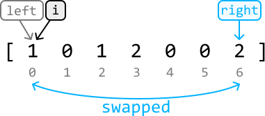
E'tibor bering, bu almashtirish keyin i indeksida yangi element paydo bo'ldi. Shuning uchun i ni hali oldinga siljitmasligimiz kerak, chunki bu yangi element boshqa joyga joylashtirilishi kerakligini hali aniqlashimiz lozim.
i ko'rsatkichi endi 1 ga ishora qilmoqda. Uchraydigan 1 larni boshqarishimiz shart emas, shuning uchun shunchaki i ko'rsatkichini oldinga siljitamiz:
![Diagram showing nums[i] == 1 condition leading to i++ action.](https://bytebytego.com/images/courses/coding-patterns/sort-and-search/dutch-national-flag/image-17-04-6-YJEWUNWU.svg?dpl=dpl_Gs7zfM6MUzjTBjcjps1LqXtb9QmD)
Endi i ko'rsatkichi 0 ga ishora qilmoqda, shuning uchun uni nums[left] bilan almashtiramiz:
![Diagram showing nums[i] == 0 condition leading to swap operation.](https://bytebytego.com/images/courses/coding-patterns/sort-and-search/dutch-national-flag/image-17-04-8-PMIDSLWB.svg?dpl=dpl_Gs7zfM6MUzjTBjcjps1LqXtb9QmD)
Bu almashtirish keyin i indeksida yangi element paydo bo'ladi. i chap ko'rsatkichdan keyin joylashganligi sababli, quyidagi sabablarga ko'ra bu element faqat 1 bo'lishi mumkin:
- Almashtirishdan oldin, i dan chapda dastlab joylashgan barcha 0 lar allaqachon chap indeksning chapiga joylashtirilgan bo'lar edi.
- Almashtirishdan oldin, i dan chapda dastlab joylashgan barcha 2 lar allaqachon o'ng indeksning o'ngiga joylashtirilgan bo'lar edi.
Shuning uchun, chap ko'rsatkichni oldinga siljitganda i ko'rsatkichini ham oldinga siljitishimiz mumkin.
Endi 0, 1 yoki 2 ga duch kelganda nima qilishni bilamiz. i ko'rsatkichi o'ng ko'rsatkichdan o'tguncha bu mantiqni qo'llashda davom etishimiz mumkin — bu barcha elementlar to'g'ri joylashtirilganligini bildiradi:

E'tibor bering, i == right bo'lganda jarayonni to'xtatmaymiz, chunki i ko'rsatkichi hali ham almashtirilishi kerak bo'lgan 0 ga ishora qilishi mumkin.
Amalga Oshirish
from typing import List
def dutch_national_flag(nums: List[int]) -> None:
i, left, right = 0, 0, len(nums) - 1
while i <= right:
# Swap 0s with the element at the left pointer.
if nums[i] == 0:
nums[i], nums[left] = nums[left], nums[i]
left += 1
i += 1
# Swap 2s with the element at the right pointer.
elif nums[i] == 2:
nums[i], nums[right] = nums[right], nums[i]
right -= 1
else:
i += 1
Murakkablik Tahlili
Vaqt murakkabligi: dutch_national_flag ning vaqt murakkabligi O(n), chunki nums ning har bir elementi bir marta o'tiladi.
Xotira murakkabligi: O(1).
Bit Manipulyatsiya
Bit Manipulyatsiyaga Kirish
Bit Manipulyatsiyaga Kirish
Intuitsiya
Bit manipulyatsiya — dasturlashda bit darajasida operatsiyalar bajarish uchun ishlatiladigan texnika bo'lib, ko'pincha yanada samarali va tez algoritmlarga olib kelishi mumkin.
Bit manipulyatsiya qachon foydali? Bit manipulyatsiya sonlarning ikkilik ifodasida to'g'ridan-to'g'ri ishlash imkonini beradi va ma'lum operatsiyalarni samaraliroq qiladi. Bit o'rnatish, tozalash, almashtirish va tekshirish kabi umumiy vazifalar bitli operatorlar yordamida tezda amalga oshirilishi mumkin.
Masalan, eng keng tarqalgan xotira optimallashtirish texnikalaridan biri — mantiqiy qiymatlar to'plamini ifodalash uchun imzosiz 32-bitli butun sondan foydalanish bo'lib, bu yerda butun sondagi har bir bit turli mantiqiy qiymatga mos keladi. Bu bizga mantiqiy massiv yoki hash set ishlatmasdan 32 tagacha holatni saqlash va boshqarish imkonini beradi.

Bitli Operatorlar
Har biri o'z maqsadiga xizmat qiluvchi bir nechta fundamental bitli operatsiyalar mavjud. Ular quyida har bir operatsiyaning haqiqat jadvali bilan ko'rsatilgan:
XOR operatorining ba'zi foydali xususiyatlari:
- a ^ 0 = a
- a ^ a = 0
Bundan tashqari, fundamental siljish operatorlarini ham tushunish muhim:
- Chapga siljish (<< n): Sonning bitlarini chapga n pozitsiyaga siljitadi, o'ngga 0 lar qo'shadi. Bu songa 2n ga ko'paytirish bilan tengdir.
- O'ngga siljish (>> n): Sonning bitlarini o'ngga n pozitsiyaga siljitadi, o'ngdagi bitlarni o'chiradi. Bu songa 2n ga bo'lish bilan tengdir (butun qismni olish).
Ushbu operatorlardan foydalanib, ba'zi foydali bit manipulyatsiya texnikalari:
- x ning i-chi bitini 1 ga o'rnatish: x |= (1 << i)
- x ning i-chi bitini 0 ga tozalash: x &= ~(1 << i)
- x ning i-chi bitini almashtirish (0 dan 1 ga yoki 1 dan 0 ga): x ^= (1 << i)
- x ning i-chi biti o'rnatilganligini tekshirish: (x >> i) & 1
- x ning eng past o'rnatilgan bitini olib tashlash: x & (x - 1)
- x ning eng past o'rnatilgan bitini ajratib olish: x & (-x)
Hayotiy Misol
Tarmoqlarda ma'lumotlar uzatish: Ko'p tarmoq protokollarida bit manipulyatsiya tezkor aloqa uchun ma'lumotlarni samarali kodlash, siqish va uzatishda qo'llaniladi. Masalan, IP manzillar va tarmoq niqoblari (subnet masks) ikkita qurilma bir xil tarmoqda ekanligini aniqlash uchun bitli AND operatsiyalaridan foydalanadi. Xuddi shunday, nazorat yig'indisi (checksum) yoki paritet bitlari kabi xatolarni aniqlash va tuzatish algoritmlarida bit manipulyatsiya ikkilik ma'lumotlardagi xatolarni aniqlab tuzatish orqali uzatish davomida ma'lumotlar yaxlitligini ta'minlaydi.
Bob Rejasi
Bit manipulyatsiya asoslarini yaxshi o'zlashtirish uchun ushbu bob bir qator murakkab bit manipulyatsiya texnikalaridan foydalanadigan turli masalalarni, shuningdek, muayyan talablar asosida tegishli bitli operatorni qanday aniqlashni o'rganadi.
Butun Sonlarning Hamming Og'irliklari
Butun Sonlarning Hamming Og'irliklari
Sonning Hamming og'irligi uning ikkilik ifodasidagi o'rnatilgan bitlar (1-bitlar) soni. Musbat n butun soni berilgan. 0 dan n gacha bo'lgan barcha i butun sonlari uchun i-chi element i butun sonining Hamming og'irligiga teng bo'lgan massiv qaytaring.
Misol:
Input: n = 7
Output: [0, 1, 1, 2, 1, 2, 2, 3]
Tushuntirish:
| Son | Ikkilik ifoda | O'rnatilgan bitlar soni |
| 0 | 0 | 0 |
| 1 | 1 | 1 |
| 2 | 10 | 1 |
| 3 | 11 | 2 |
| 4 | 100 | 1 |
| 5 | 101 | 2 |
| 6 | 110 | 2 |
| 7 | 111 | 3 |
Intuitsiya - Har Bir Son Uchun Bitlarni Sanash
Eng oddiy strategiya — 0 dan n gacha bo'lgan har bir son uchun bitlar sonini alohida sanash.
x = 25 soni va uning ikkilik ifodasini ko'rib chiqaylik:

Sondagi o'rnatilgan bitlar (1 lar) sonini hisoblash uchun har bir bitni tekshirib, o'rnatilgan bit topganda hisoblagichni oshirishimiz mumkin.
x ning LSB (eng muhim bo'lmagan bit) ni tekshirish uchun AND operatorini 1 bilan ishlatishimiz mumkin: x & 1. Agar natija 1 bo'lsa, LSB o'rnatilgan.
Keyingi bitni qanday tekshiramiz? x da bitli o'ngga siljish operatsiyasini bajarsak, x ning barcha bitlari bir pozitsiya o'ngga siljiydi. Bu keyingi bitni yangi LSB qilib qo'yadi:
Endi sondagi o'rnatilgan bitlar sonini hisoblash uchun takrorlashimiz mumkin bo'lgan jarayon bor:
- x & 1 yordamida x ning LSB ni tekshiring va agar 1 bo'lsa hisoblagichni oshiring.
- x ni o'ngga siljiting.
x 0 ga tengligacha yuqoridagi ikki qadamni davom eting — bu sanash uchun o'rnatilgan bitlar qolmaganligini bildiradi. Buni 0 dan n gacha bo'lgan har bir son uchun bajarish javobni beradi.
Amalga Oshirish - Har Bir Son Uchun Bitlarni Sanash
from typing import List
def hamming_weights_of_integers(n: int) -> List[int]:
result = []
for i in range(n + 1):
count = 0
x = i
while x:
count += x & 1
x >>= 1
result.append(count)
return result
Murakkablik Tahlili
Vaqt murakkabligi: hamming_weights_of_integers ning vaqt murakkabligi O(n log(n)), chunki 0 dan n gacha bo'lgan har bir x butun soni uchun o'rnatilgan bitlarni sanash logarifmik vaqt oladi, chunki ushbu sonda taxminan log2(x) bit mavjud. Barcha butun sonlar 32 bitga ega deb faraz qilsak, vaqt murakkabligi O(n) ga soddalashadi.
Xotira murakkabligi: O(1), chunki natija egallagan joydan tashqari qo'shimcha joy ishlatilmaydi.
Intuitsiya - Dinamik Dasturlash
Oldingi yondashuvda, x butun soniga yetib borganимизда 0 dan x - 1 gacha bo'lgan barcha butun sonlar uchun natijani allaqachon hisoblaganligimizni ta'kidlash muhim. Agar bu oldingi natijalardan foydalanish usulini topsak, natija massivini tuzishning samaradorligini oshirishimiz mumkin.
0 dan x - 1 gacha bo'lgan butun sonlarning natijalarini x ning potensial kichik masalalari sifatida ko'rib optimal kichik tuzilmadan foydalanish usulini topish maqsadga muvofiq. Bu DP yechimining boshlanishi. dp[x] x butun sonidagi o'rnatilgan bitlar sonini ifodalaydi.
dp[x] ning kichik masalasiga oldindan aytish mumkin bo'lgan kirish usuli — x ni 1 ga o'ngga siljitish va LSB ni samarali olib tashlash. Bu dp[x >> 1] kichik masalasi bo'lib, u va dp[x] o'rtasidagi yagona farq — hozirgina olib tashlangan LSB.
Ilgari aytilganidek, x ning LSB x & 1 yordamida topilishi mumkin. Shuning uchun:
- Agar x ning LSB 0 bo'lsa, x va x >> 1 o'rtasida bitlar sonida farq yo'q:
- Agar x ning LSB 1 bo'lsa, x va x >> 1 o'rtasida bitlar sonidagi farq 1 ga teng:
Shuning uchun, dp[x >> 1] natijasini olib unga LSB ni qo'shish orqali dp[x] ni olishimiz mumkin:
dp[x] = dp[x >> 1] + (x & 1)
Endi asosiy holat nima ekanligini bilishimiz kerak.
Asosiy holat Bu masalaning eng oddiy versiyasi n 0 ga teng bo'lganda. Bu holda o'rnatilgan bitlar yo'q, shuning uchun o'rnatilgan bitlar soni 0. Bu asosiy holatni dp[0] ni 0 ga o'rnatish orqali qo'llashimiz mumkin.
Asosiy holat o'rnatilgandan so'ng, DP massivining qolgan qismini dp[1] dan dp[n] gacha formulamizni qo'llab to'ldiramiz. Masalaning javobi esa 0 dan n gacha bo'lgan har bir son uchun o'rnatilgan bitlar sonini o'z ichiga olgan DP massivi qiymatlari bo'ladi.
Amalga Oshirish - Dinamik Dasturlash
from typing import List
def hamming_weights_of_integers_dp(n: int) -> List[int]:
dp = [0] * (n + 1)
for i in range(1, n + 1):
dp[i] = dp[i >> 1] + (i & 1)
return dp
Murakkablik Tahlili
Vaqt murakkabligi: hamming_weights_of_integers_dp ning vaqt murakkabligi O(n), chunki DP massivining har bir elementini bir marta to'ldiramiz.
Xotira murakkabligi: O(1), chunki bu holda DP massivi bo'lgan natija egallagan joydan tashqari qo'shimcha joy ishlatilmaydi.
Yolg'iz Butun Son
Yolg'iz Butun Son
Bittasidan tashqari har bir son ikki marta takrorlanadigan butun sonlar massivi berilgan. Noyob sonni toping.
Misol:
Input: nums = [1, 3, 3, 2, 1]
Output: 2
Cheklovlar:
- nums kamida bitta elementdan iborat.
Intuitsiya
Hash map yechimi Bu masalani hal qilishning oddiy usuli — hash map dan foydalanish. G'oya — massivdagi har bir elementning takrorlanish sonini hisoblash. Buni massiv bo'ylab o'tib, uchraydigan har bir elementning hash map dagi chastotasini oshirish orqali amalga oshirishimiz mumkin.
![Hash map approach: nums=[1,3,3,2,1], hashmap shows {1:2, 2:1, 3:2}, lonely integer is 2.](https://bytebytego.com/images/courses/coding-patterns/bit-manipulation/lonely-integer/image-18-02-1-M2A4JCS6.svg?dpl=dpl_Gs7zfM6MUzjTBjcjps1LqXtb9QmD)
To'ldirilgandan so'ng, chastotasi 1 bo'lgan elementni topish uchun hash map ni ko'rib chiqishimiz mumkin — bu bizning yolg'iz butun sonimiz. Bu yondashuv O(n) vaqt oladi, lekin O(n) xotira sarflanadi, bu yerda n kirish massivining uzunligini bildiradi. Hash map kabi qo'shimcha ma'lumotlar strukturalari ishlatmasdan hal qilish usuli bormi?
Saralash yechimi Boshqa usul — massivni avval saralashtirish, keyin esa massiv bo'ylab o'tib har bir elementni qo'shnilari bilan taqqoslash orqali yolg'iz butun sonni qidirish. Yolg'iz butun son — yonida dublikati bo'lmagan element.
![Sorting solution: [1,3,3,2,1] sorted to [1,1,2,3,3], 2 has no duplicates next to it.](https://bytebytego.com/images/courses/coding-patterns/bit-manipulation/lonely-integer/image-18-02-2-KHYDB73Q.svg?dpl=dpl_Gs7zfM6MUzjTBjcjps1LqXtb9QmD)
Bu usul saralash tufayli O(n log(n)) vaqt oladi, lekin saralash vaqtida ishlatilganlardan tashqari qo'shimcha ma'lumotlar strukturasi talab qilmaydigan afzallikka ega. Chiziqli vaqt murakkabligini saqlab va doimiy xotiradan foydalangan holda hal qilish usuli bormi?
Bit manipulyatsiya Qo'shimcha xotira ishlatishdan qochishning bir usuli — bit manipulyatsiya. XOR operatsiyasi, ayniqsa, takroriy butun sonlarni boshqarishda foydali bo'lishi mumkin. XOR operatorining quyidagi ikki xususiyatini esga oling:
- a ^ a == 0
- a ^ 0 == a
Ko'rib turganimizdek, ikkita bir xil sonni XOR qilganimizda natija 0 bo'ladi. Yolg'iz butun sondan tashqari har bir son massivda ikki marta paydo bo'lganligi sababli, barcha sonlarni XOR qilsak, bir xil sonlarning barcha juftliklari 0 ga qisqaradi. Bu yolg'iz butun sonni ajratib beradi: barcha takroriy elementlar 0 ga qisqaргandan so'ng, 0 ni yolg'iz butun son bilan XOR qilish bizga yolg'iz butun sonni beradi.
Bu sonlarning massivda qayerda joylashganidan mustaqil ishlaydi, chunki XOR kommutativlik va assotsiativlik xususiyatlariga amal qiladi:
- Kommutativlik xususiyati: a ^ b == b ^ a
- Assotsiativlik xususiyati: (a ^ b) ^ c == a ^ (b ^ c)
Shunday qilib, massivda bir xil ikkita son mavjud bo'lsa, barcha elementlarni XOR qilganimizda ular bekor bo'ladi. Buning misoli quyida ko'rsatilgan:
Bu qo'shimcha xotira ishlatmasdan chiziqli vaqtda yolg'iz butun sonni aniqlash imkonini beradi.
Amalga Oshirish
from typing import List
def lonely_integer(nums: List[int]) -> int:
res = 0
# XOR each element of the array so that duplicate values will cancel each other
# out (x ^ x == 0).
for num in nums:
res ^= num
# 'res' will store the lonely integer because it would not have been canceled out
# by any duplicate.
return res
Murakkablik Tahlili
Vaqt murakkabligi: lonely_integer ning vaqt murakkabligi O(n), chunki nums dagi har bir elementda doimiy vaqt oladigan XOR operatsiyasini bajaramiz.
Xotira murakkabligi: O(1).
Toq va Juft Bitlarni Almashtirish
Toq va Juft Bitlarni Almashtirish
Imzosiz 32-bitli n butun soni berilgan. n ning barcha juft bitlari qo'shni toq bitlari bilan almashtirilgan butun sonni qaytaring.
-Misol:

Input: n = 41
Output: 22
-Misol:

Input: n = 23
Output: 43
Intuitsiya
Juft va toq bitlarni almashtirish — juft pozitsiyadagi har bir bit keyingi toq pozitsiyadagi bit bilan almashtirilishi va aksincha. E'tibor bering, pozitsiyalar 0 dan boshlanadi, bu eng muhim bo'lmagan bitning pozitsiyasi.
Almashtirish uchun e'tibor berilishi kerak bo'lgan asosiy narsa:
- Juft pozitsiyadagi barcha bitlar bir pozitsiya chapga siljitilishi kerak.
- Toq pozitsiyadagi barcha bitlar bir pozitsiya o'ngga siljitilishi kerak.
Bu juft va toq pozitsiyadagi barcha bitlarni alohida ajratib olish usuli bo'lsa, ularni mos ravishda siljitib, keyin birlashtirish mumkinligini bildiradi — shunda toq pozitsiyadagi bitlar juft pozitsiyalarda, aksincha bo'ladi.
n ning juft va toq bitlarini qanday olishni aniqlab olaylik.
Barcha juft bitlarni olish n ning barcha juft bitlarini olish uchun barcha juft bit pozitsiyalari 1 ga o'rnatilgan niqob (mask) ishlatishimiz mumkin:

Bu niqob va n bilan bitli AND bajarish toq pozitsiyadagi barcha bitlar 0 ga o'rnatilgan, faqat n ning juft pozitsiyadagi bitlari saqlanadigan butun son beradi:

Barcha toq bitlarni olish Xuddi shunday, n ning barcha toq bitlarini olish uchun barcha toq bit pozitsiyalari 1 ga o'rnatilgan niqob ishlatishimiz mumkin:

Bu niqob va n bilan bitli AND bajarish juft pozitsiyadagi barcha bitlar 0 ga o'rnatilgan, faqat n ning toq pozitsiyadagi bitlari saqlanadigan butun son beradi:

Barcha juft va toq bitlarni alohida ajratib olgandan so'ng, toq va juft pozitsiyadagi bitlar almashtirilgan natijani olish uchun ulardan foydalanamiz.
Toq va juft pozitsiyadagi bitlarni siljitish va birlashtirish Siljish operatoridan juft pozitsiyadagi bitlarni bir marta chapga, toq pozitsiyadagi bitlarni bir marta o'ngga siljitish uchun foydalanishimiz mumkin:
Keyin ularni birlashtirish uchun bitli OR operatoridan foydalanishimiz mumkin, chunki u ikki to'plam bitni yakuniy natijaga birlashtiradi.

Endi toq pozitsiyadagi bitlar juft pozitsiyalarda va aksincha.
Amalga Oshirish
def swap_odd_and_even_bits(n: int) -> int:
# Mask to extract even bits (positions 0, 2, 4, ...): 0x55555555 = 01010101...
even_mask = 0x55555555
# Mask to extract odd bits (positions 1, 3, 5, ...): 0xAAAAAAAA = 10101010...
odd_mask = 0xAAAAAAAA
# Extract even bits and shift left, extract odd bits and shift right
even_bits = (n & even_mask) << 1
odd_bits = (n & odd_mask) >> 1
# Merge the two
return even_bits | odd_bits
Murakkablik Tahlili
Vaqt murakkabligi: swap_odd_and_even_bits ning vaqt murakkabligi O(1).
Xotira murakkabligi: O(1).
Matematika va Geometriya
Matematika va Geometriyaga Kirish
Matematika va Geometriyaga Kirish
Intuitsiya
Ushbu bob dasturlashda texnik suhbatlarda muntazam uchraydigan muhim matematika va geometriya kontseptsiyalariga oid bir nechta masalalarni ko'rib chiqadi.
Biz quyidagi mavzularni o'rganamiz:
- Eng katta umumiy bo'luvchi (EKUB).
- Modul arifmetikasi.
- Suzuvchi nuqta aniqligini boshqarish.
- Butun son to'lib ketishi va kamayib ketishini boshqarish.
- Naqshlarni aniqlash.
Hayotiy Misol
Kompyuter grafikasi: 3D renderlashda geometriya ob'ektlarni ko'pburchak kabi shakllar sifatida ifodalash uchun ishlatiladi va bu ob'ektlarni animatsiya qilish yoki ularning perspektivasini o'zgartirish uchun aylantirish, kengaytirish va ko'chirish kabi matematik transformatsiyalar qo'llaniladi. Trigonometriya, vektor matematikasi va matritsa operatsiyalaridan foydalanadigan algoritmlar virtual muhitlarda ob'ektlarning qanday harakat qilishini, yorug'lik bilan qanday o'zaro ta'sirda bo'lishini yoki soya qanday tushishini aniqlashda muhim rol o'ynaydi.
Bob Rejasi
Spiral Tartibida O'tish
Spiral Tartibida O'tish
Matritsaning elementlarini soat yo'nalishida spiral tartibida qaytaring.
Misol:
Output: [0, 1, 2, 3, 4, 9, 14, 19, 18, 17, 16, 15, 10, 5, 6, 7, 8, 13, 12, 11]
Intuitsiya
Bu masala uchun kutilgan natijani yaratish uchun masala tavsifini to'liq simulyatsiya qilib, matritsani spiral tartibida o'tishga harakat qilaylik va har bir qiymatni o'tganimizda natijaga qo'shamiz. Buni qanday qilish mumkin?
Spiral tartibida o'tish — matritsani bitta yo'nalishda borishni davom ettirish mumkin bo'lmagan joyga yetguncha siljish, keyin yo'nalishni o'zgartirish va davom ettirishni o'z ichiga oladi. Xususan, yo'nalishlar ketma-ketligi — o'ng, pastga, chapga va yuqoriga — barcha elementlar o'tilguncha takrorlanadi. Buni amalga oshirish uchun yo'nalishlarni almashtirish uchun aniq shartlarni aniqlashimiz kerak.
Dastlab yondashuvimiz oddiy tuyulishi mumkin: matritsaning o'ng chegarasiga yetguncha o'ngga siljishdan boshlaymiz, shunda yo'nalishni o'zgartiramiz. Buni uch marta muammosiz harakatlanib yo'nalishni o'zgartirishimiz mumkin:
Biroq, quyida ko'rsatilganidek, matritsaning yuqori qatoriga yetguncha yuqoriga harakat qilsak, boshlaganimiz joyga qaytamiz va ilgari tashrif buyurilgan katakdagi qiymatni natijaga qo'shamiz:
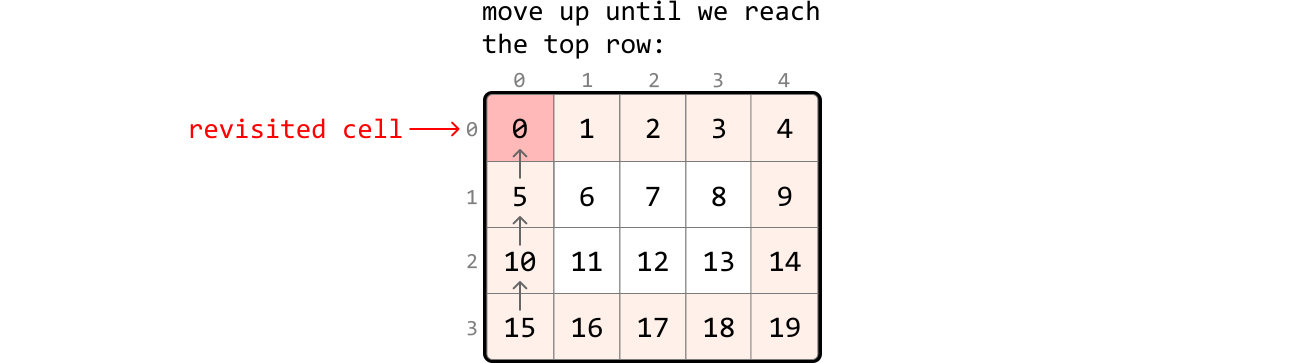
Buning mumkin bo'lgan yechimi — barcha tashrif buyurilgan kataklar hash set yordamida kuzatib borish. Bu bizga ilgari ko'rilgan katakka duch kelganda o'sha yo'nalishda to'xtashimizga imkon beradi. Ushbu yondashuv samarali bo'lsa-da, O(m*n) xotira talab qiladi. Qo'shimcha ma'lumotlar strukturasisiz oldin tashrif buyurilgan kataklar qayta ko'rilmasligini ta'minlash mumkinmi?
Yuqoridagi rasmlarda e'tibor bering: ma'lum yo'nalishda harakat qilganimizda chegara satr yoki ustunga (ya'ni yuqori yoki pastki satr, yoki eng chap yoki eng o'ng ustun) yetguncha davom ettiramiz.
Nima bo'ladi, agar biz matritsani o'tib chiqqanimizda ushbu chegaralarni ilgari o'tilgan kataklar qayta ko'rilmasligi uchun moslashtirsak?
Chegaralarni moslashtirish To'rtta chegarani (yuqori, pastki, chap, o'ng) boshlang'ich pozitsiyalari bilan ishga tushiramiz:
- top = 0
- bottom = m - 1
- left = 0
- right = n - 1
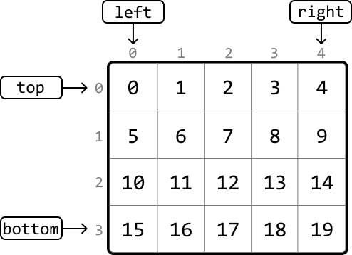
Birinchi qatorni chap chegaradan o'ngga o'tib o'tishni boshlaymiz. Birinchi qatordagi barcha kataklar tashrif buyurilganligi sababli bu qatorga keyingi kirishni oldini olishimiz kerak. Buni yuqori chegarani 1 ga pastga siljitish (top += 1) orqali amalga oshirishimiz mumkin, bu esa yuqori qatorga kira olmasligimizni ta'minlaydi:
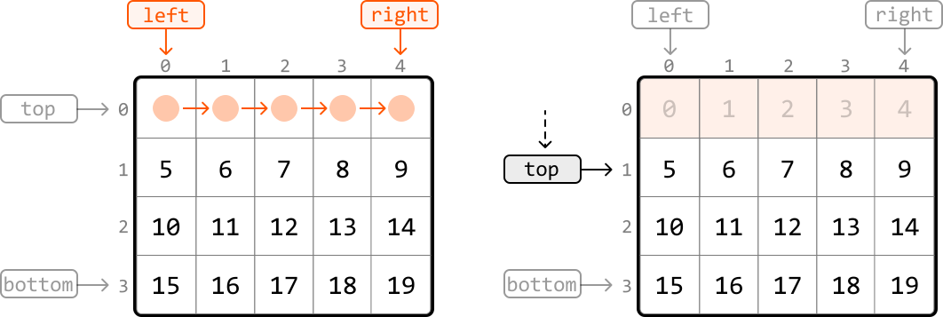
Keyin, yuqori chegaradan pastki chegaraga pastga siljitamiz. Bu ustun qayta ko'rilmasligini ta'minlash uchun o'ng chegarani yangilang (right -= 1):
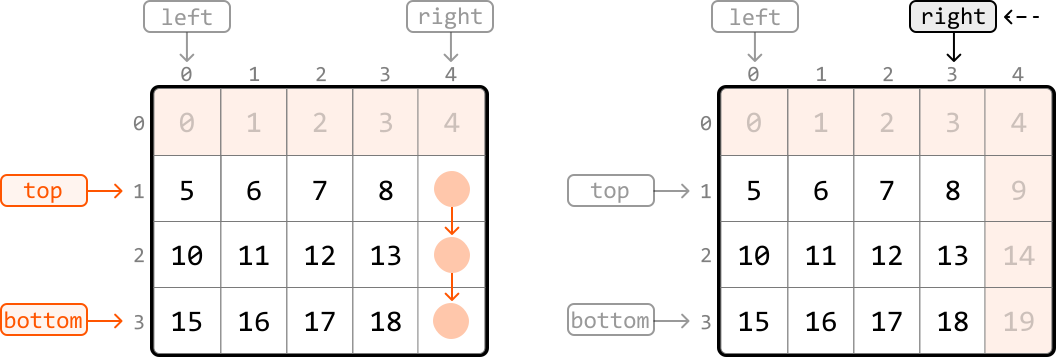
Keyin, o'ng chegaradan chapga chapga siljitamiz. Bu satr qayta ko'rilmasligini ta'minlash uchun pastki chegarani yangilang (bottom -= 1):
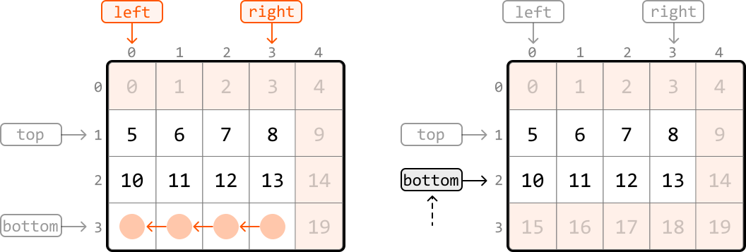
Keyin, pastki chegaradan yuqori chegaraga yuqoriga siljitamiz. Bu ustun qayta ko'rilmasligini ta'minlash uchun chap chegarani yangilang (left += 1):
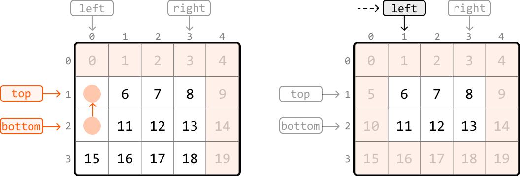
To'rtta yo'nalishning har birida qanday o'tish va mos chegaralarni yangilashni muhokama qildik. Bu o'tishlar yuqori chegara pastki chegaradan o'tib ketmaguncha yoki chap chegara o'ng chegaradan o'tib ketmaguncha takrorlanadi. Ularning ikkalasi ham o'tish uchun kataklarning qolmaganligini bildiradi.
Xulosa qilib aytganda, matritsani spiral tartibida o'tish uchun quyidagi o'tishlar ketma-ketligini takrorlaymiz:
- Yuqori chegara bo'ylab chapdan o'ngga harakat qilish, keyin yuqori chegarani yangilash (top += 1)
- O'ng chegara bo'ylab yuqoridan pastga harakat qilish, keyin o'ng chegarani yangilash (right -= 1)
- Pastki chegara bo'ylab o'ngdan chapga harakat qilish, keyin pastki chegarani yangilash (bottom -= 1)
- Chap chegara bo'ylab pastdan yuqoriga harakat qilish, keyin chap chegarani yangilash (left += 1)
Bu top <= bottom va left <= right bo'lguncha davom etadi.
Yodda tutish kerak bo'lgan muhim narsa: yuqori chegarani yangilagandan so'ng, yuqori chegara pastki chegaradan o'tib ketishi mumkin (top > bottom). Shuning uchun pastki chegara bo'ylab o'tishdan oldin top <= bottom ekanligini tekshirishimiz kerak. Xuddi shunday, chegaralar kesishib ketmaganligini ta'minlash uchun chap chegara bo'ylab o'tishdan oldin left <= right ekanligini tekshirishimiz kerak.
Matritsani o'tib chiqqanimizda uchraydigan har bir qiymatni natija massiviga qo'shamiz. Shunday qilib, matritsaning qiymatlari spiral tartibida qayd etiladi.
Amalga Oshirish
from typing import List
def spiral_matrix(matrix: List[List[int]]) -> List[int]:
if not matrix:
return []
result = []
# Initialize the matrix boundaries.
top, bottom = 0, len(matrix) - 1
left, right = 0, len(matrix[0]) - 1
# Traverse the matrix in spiral order.
while top <= bottom and left <= right:
# Move from left to right along the top boundary.
for i in range(left, right + 1):
result.append(matrix[top][i])
top += 1
# Move from top to bottom along the right boundary.
for i in range(top, bottom + 1):
result.append(matrix[i][right])
right -= 1
# Check that the bottom boundary hasn't passed the top boundary before
# moving from right to left along the bottom boundary.
if top <= bottom:
for i in range(right, left - 1, -1):
result.append(matrix[bottom][i])
bottom -= 1
# Check that the left boundary hasn't passed the right boundary before
# moving from bottom to top along the left boundary.
if left <= right:
for i in range(bottom, top - 1, -1):
result.append(matrix[i][left])
left += 1
return result
Murakkablik Tahlili
Vaqt murakkabligi: spiral_matrix ning vaqt murakkabligi O(m*n), chunki matritsaning har bir katagi bir marta o'tiladi.
Xotira murakkabligi: O(1). res massivi xotira murakkabligiga kirmaydi.
32-Bitli Butun Sonni Teskari Yozish
-Bitli Butun Sonni Teskari Yozish
Imzolangan 32-bitli butun sonning raqamlarini teskari tartibda yozing. Agar teskari yozilgan butun son to'lib ketsa (ya'ni [-2^31, 2^31 - 1] diapazonidan tashqarida bo'lsa), 0 ni qaytaring. Muhit faqat imzolangan 32-bitli butun son diapazonidagi butun sonlarni saqlashga ruxsat beradi deb faraz qiling.
-Misol:
Input: n = 420
Output: 24
-Misol:
Input: n = -15
Output: -51
Intuitsiya
Bu masaladagi asosiy qiyinlik — chekka holatllarni boshqarish. Bu chekka holatllarni hal qilishdan oldin, avval oddiyroq holatlarni ko'rib chiqaylik va keyin strategiyamizni qanday o'zgartirishimiz kerakligini ko'ramiz.
Musbat sonlarni teskari yozish n = 123 ni ko'rib chiqaylik. Teskari yozilgan butun sonni bir vaqtda bir raqam qurishga harakat qilaylik. Eng avval raqamlarimizni qurish uchun n ning raqamlari bo'ylab qanday o'tishni aniqlash kerak (dastlab 0 ga o'rnatilgan):

Buni n ning oxirgi raqamidan boshlab har bir raqamni reversed_n ga qo'shib o'tish orqali amalga oshirish mumkin:
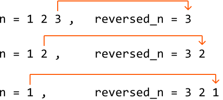
Buni qanday amalga oshirish mumkinligini o'rganaylik. Oxirgi raqamni ajratib olish uchun modul operatoridan foydalanishimiz mumkin: n % 10. Bu amaliyot n ni 10 ga bo'lgandagi qoldiqni topadi:
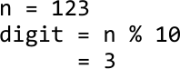
Oxirgi raqamni ajratib olgandan so'ng, n ni 10 ga bo'lib uni olib tashlaymiz, bu ikkinchi oxirgi raqamni oxirgi pozitsiyaga siljitadi va keyingi iteratsiyaga tayyorlaydi:
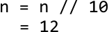
Shundan so'ng, ajratib olingan oxirgi raqamni teskari sonimizga qo'shamiz:

Keyingi raqamni qayta ishlash uchun modul amaliyoti yordamida n dan ajratib olaylik, keyin n ni 10 ga bo'lib uni olib tashlaymiz:
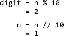
Bu raqamni reversed_n ga qo'shish uchun reversed_n ni 10 ga ko'paytirib uning raqamlarini chapga siljitishimiz va yangi raqam uchun joy ochishimiz mumkin. Keyin avvalgidek yangi raqamni qo'shamiz:

n ning barcha raqamlari reversed_n ga qo'shilguncha (ya'ni n 0 ga tengligacha) yuqoridagi jarayonni takrorlashimiz mumkin. Bu jarayonning qisqacha bayoni:
- Oxirgi raqamni ajratib olish: digit = n % 10.
- Oxirgi raqamni olib tashlash: n = n // 10.
- Raqamni qo'shish: reversed_n = reversed_n * 10 + digit.
Manfiy sonlarni teskari yozish Manfiy sonlarni boshqarish uchun alohida strategiyani ko'rib chiqishdan oldin, avval yuqoridagi qadamlar manfiy sonlarda ham ishlashini tekshiraylik. Bu qadamlarni n = -15 ga qo'llash:
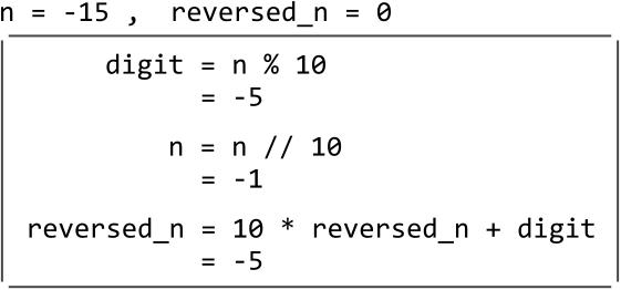
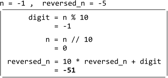
Ko'rib turganimizdek, manfiy sonlarda ham ishlaydi. Endi sonni teskari yozish butun son to'lib ketishi yoki kamayib ketishiga olib kelishi mumkin bo'lgan holatllarni ko'rib chiqaylik.
Butun son to'lib ketishini aniqlash Agar musbat sonning teskarisi 2^31 - 1 dan katta bo'lsa, u to'lib ketadi va 0 qaytarishimiz kerak. Bu maksimal qiymatni INT_MAX deb ataymiz.

Dastlab sonni to'liq teskari yozish, 2^31 - 1 dan oshib ketishini tekshirish va oshib ketsa 0 qaytarish yetarli tuyulishi mumkin. Biroq, 2^31 - 1 dan katta butun sonlar saqlab bo'lmaydigan muhitda bunday butun sonni teskari yozishga urinish to'lib ketishiga olib keladi:

Shuning uchun to'lib ketishni aniqlashning boshqa usulini o'ylab topaylik.
Biz reversed_n ni bir vaqtda bir raqam qurmoqdamiz, bu har bir yangi qo'shadigan raqam bilan son to'lib ketmasligi uchun chora ko'rishimiz kerakligini anglatadi. Yangi raqam qo'shish reversed_n ni haddan oshib ketishiga qachon olib kelishi mumkinligini o'ylab ko'raylik. Buni quyidagicha tahlil qilishimiz mumkin:
Agar reversed_n 214748364 ga teng bo'lsa (ya'ni INT_MAX // 10), to'lib ketishdan qochish uchun unga qo'shilishi mumkin bo'lgan yakuniy raqam 7 dan kichik yoki teng bo'lishi kerak (chunki 2147483647 == INT_MAX):


Endi yodda tuting: reversed_n == INT_MAX // 10 bo'lganda, unga faqat bitta raqam qo'shilishi mumkin. Bu yerda asosiy kuzatuv shundaki, bu raqam faqat 1 bo'lishi mumkin, chunki kattaroq yakuniy raqam imkonsiz bo'lar edi:

Bu reversed_n == INT_MAX // 10 bo'lganda, unga qo'shiladigan oxirgi raqam to'lib ketishga olib kelmasligini anglatadi — demak bu holda oxirgi raqamni tekshirishimiz shart emas.
Agar reversed_n allaqachon INT_MAX // 10 dan katta bo'lsa, istalgan raqam qo'shish to'lib ketishiga olib keladi. Bu holatni quyidagi shart bilan boshqarishimiz mumkin:
if reversed_n > INT_MAX // 10: return 0
Butun son kamayib ketishini aniqlash Yuqoridagiga o'xshash mantiqni butun son kamayib ketishini boshqarish uchun ham qo'llashimiz mumkin. Bu yerda reversed_n ning INT_MIN // 10 dan pastga tushmasligini tekshirishimiz kerak:
if reversed_n < INT_MIN // 10: return 0
Amalga Oshirish
Python-da manfiy son bilan modul operatoridan (%) foydalanish musbat natija beradi. Bundan qochish uchun math.fmod dan foydalanib, uning natijasini manfiy modul qiymatiga ega bo'lish uchun butun songa o'tkazishimiz mumkin.
Bo'lish uchun Python-ning // operatori pastki bo'lish (floor division) ni amalga oshiradi, bu manfiy sonlar bilan ishlashda kerakli bo'lmagan qiymat hosil qilishi mumkin (masalan, -15 // 10 kerakli -1 o'rniga -2 beradi). Kerakli xulq-atvorga erishish uchun bo'lish uchun / dan foydalaning va natijasini butun songa o'tkazing.
import math
def reverse_32_bit_integer(n: int) -> int:
INT_MAX = 2**31 - 1
INT_MIN = -2**31
reversed_n = 0
# Keep looping until we've added all digits of 'n' to 'reversed_n' in reverse
# order.
while n != 0:
# digit = n % 10
digit = int(math.fmod(n, 10))
# n = n // 10
n = int(n / 10)
# Check for integer overflow or underflow.
if reversed_n > int(INT_MAX / 10) or reversed_n < int(INT_MIN / 10):
return 0
# Add the current digit to 'reversed_n'.
reversed_n = reversed_n * 10 + digit
return reversed_n
Murakkablik Tahlili
Vaqt murakkabligi: reverse_32_bit_integer ning vaqt murakkabligi O(log(n)), chunki n ning har bir raqami bo'ylab o'tamiz, ular taxminan log(n) ta raqamdan iborat. Bu muhit faqat 32-bitli butun sonlarni qo'llab-quvvatlaganligi sababli, vaqt murakkabligi O(1) sifatida ham qaralishi mumkin.
Xotira murakkabligi: O(1).
Maksimal Kollinear Nuqtalar
Maksimal Kollinear Nuqtalar
Ikki o'lchamli tekislikdagi nuqtalar to'plami berilgan. Bir to'g'ri chiziqda joylashgan maksimal nuqtalar sonini aniqlang.
Misol:
Input: points = [[1, 1], [1, 3], [2, 2], [3, 1], [3, 3], [4, 4]]
Output: 4
Cheklovlar:
- Kirish takroriy nuqtalarni o'z ichiga olmaydi.
Intuitsiya
Ikki yoki undan ko'p nuqta bir to'g'ri chiziqda joylashgan bo'lsa, ular kollinear. Boshqacha aytganda, ular orasidagi istalgan nuqtalar juftligi o'rtasidagi qiyalik teng bo'ladi:
Ikki nuqta (xa, ya) va (xb, yb) berilganda chiziq qiyaligini qanday hisoblanishini eslaymiz:
qiyalik = ko'tarilish / yugurish = (yb - ya) / (xb - xa)
Ushbu formuladan foydalanib, kirishdagi barcha nuqtalar juftliklari o'rtasidagi qiyalikni hisoblab, bir xil qiyalikni bo'lishuvchi eng ko'p juftliklar sonini aniqlaymiz. Biroq, bu yondashuv nuqsonli, chunki bir xil qiyalikka ega bo'lgan ikki nuqtalar juftligi kollinear bo'lmasligi mumkin:
Javobni topishning boshqa usulini o'ylab ko'raylik. Muayyan nuqta bilan kollinear bo'lgan maksimal nuqtalar sonini topishga harakat qilsak nima bo'ladi? Bu nuqtani fokal nuqta deb ataymiz.
Fokal nuqta va kirimdagi har bir boshqa nuqta o'rtasidagi qiyalikni hisoblab, har bir qiyalik qiymatiga nechta nuqta mos kelishini hash map yordamida sanashimiz mumkin. E'tibor bering, hash map da saqlanadigan nuqtalar chastotalari fokal nuqtani o'z ichiga olmaydi.
Bu fokal nuqta bilan kollinear bo'lgan maksimal nuqtalar sonini topishimizga imkon beradi:
Bu yerda eng yuqori chastotali qiyalik 3 ga teng, ya'ni ushbu qiyalik bilan belgilangan chiziqda nuqtalar soni 3 + 1 = 4, bu yerda +1 fokal nuqtaning o'zini hisobga oladi.
Har bir nuqta uchun jarayonni takrorlab, har bir fokal nuqta bilan kollinear bo'lgan maksimal nuqtalar sonini aniqlashimiz mumkin. Yakuniy javobimiz ushbu maksimumlarning eng kattasiga teng.
Chekka holat: bir x-o'qida ikkita nuqta Ikki kollinear nuqta bir x-o'qini bo'lishganda, qiyalik formulasining maxraji 0 ga teng bo'ladi. Bu muammo, chunki 0 ga bo'lish noaniq:
Bu muammoni hal qilish uchun yugurish qiymati 0 ga teng ekanligini tekshirishimiz mumkin. Shunday bo'lsa, ushbu qiyalik qiymatini ifodalash uchun cheksizlikdan (float('inf')) foydalanishimiz mumkin.
Aniqlik muammolaridan qochish Qiyaliklarni float yoki double sifatida saqlaganda ularning aniqligi haqida diqqatli bo'lish zarur. Quyidagi qiyaliklarni ko'rib chiqaylik:
Ko'rib turganimizdek, kasrlarning o'zi turli qiyaliklarni ifodalaса-da, ularni float yoki double sifatida taqdim etish ularni aniq farqlash uchun yetarli o'nli kasr aniqligini ta'minlamaydi. Bu turli qiyaliklarni bir xil deb noto'g'ri aniqlashga olib kelishi mumkin.
Bundan qochish uchun qiyalikni tuple sifatida saqlangan bir juft butun son sifatida ifodalashimiz mumkin: (ko'tarilish, yugurish). Masalan, ko'tarilishi 1 va yugurishi 2 bo'lgan qiyalik 1 / 2 = 0.5 o'rniga (1, 2) sifatida ifodalanishi mumkin.
Qiyaliklarning izchil ifodalanishini ta'minlash Hal qilish kerak bo'lgan yana bitta qiyinlik bor: teng qiyalik kasr uchun ifodalanishning barcha ekvivalent qiyalik kasrlar uchun izchil bo'lishini ta'minlash:
Kasrlarni eng sodda ko'rinishga kamaytirsak, turli boshlang'ich ifodalarga ega teng kasrlarni izchil ifodalashimiz mumkin.
Lekin buni qanday qilish mumkin? Ko'tarilish va yugurish ikkalasini ularning eng katta umumiy bo'luvchisiga (EKUB) bo'lish orqali kasrlarni kamaytirish mumkin.
Eng katta umumiy bo'luvchi Ikki sonning EKUB — ikkisini ham qoldiqsiz bo'ladigan eng katta son. Ko'tarilish va yugurish ni EKUB ga bo'lish qiyalikni eng sodda ko'rinishga kamaytiradi:

Bu barcha teng kasrlar bir xil tarzda ifodalanishini ta'minlaydi.
Amalga Oshirish
from typing import List, Tuple
from collections import defaultdict
def maximum_collinear_points(points: List[List[int]]) -> int:
res = 0
# Treat each point as a focal point, and determine the maximum number of points
# that are collinear with each focal point. The largest of these maximums is the
# answer.
for i in range(len(points)):
res = max(res, max_points_from_focal_point(i, points))
return res
def max_points_from_focal_point(focal_point_index: int, points: List[List[int]]) -> int:
slopes_map = defaultdict(int)
max_points = 0
# For the current focal point, calculate the slope between it and every other
# point. This allows us to group points that share the same slope.
for j in range(len(points)):
if j != focal_point_index:
curr_slope = get_slope(points[focal_point_index], points[j])
slopes_map[curr_slope] += 1
# Update the maximum count of collinear points for the current focal
# point.
max_points = max(max_points, slopes_map[curr_slope])
# Add 1 to max_points to account for the focal point itself.
return max_points + 1
def get_slope(point_a: List[int], point_b: List[int]) -> Tuple[int, int]:
rise = point_b[1] - point_a[1]
run = point_b[0] - point_a[0]
# Handle vertical lines.
if run == 0:
return (1, 0)
# Reduce the slope fraction to its simplest form.
common_divisor = gcd(abs(rise), abs(run))
# Normalize the sign of the slope.
sign = -1 if (rise < 0) != (run < 0) else 1
return (sign * abs(rise) // common_divisor, abs(run) // common_divisor)
def gcd(a: int, b: int) -> int:
while b != 0:
a, b = b, a % b
return a
Ba'zi dasturlash tillari, jumladan Python ham, EKUB funksiyasining o'z ichki amalga oshirilishiga ega bo'lsa-da, uning amalga oshirilishi ma'lumot uchun quyida keltirilgan. Bu amalga oshirish odatda Evklid algoritmi nomi bilan tanilgan:
# The Euclidean algorithm.
def gcd(a, b):
while b != 0:
a, b = b, a % b
return a
Murakkablik Tahlili
Vaqt murakkabligi: maximum_collinear_points ning vaqt murakkabligi O(n^2 * log(m)), bu yerda n nuqtalar sonini, m esa koordinatalar orasidagi eng katta qiymatni bildiradi.
- gcd(rise, run) funksiyasining vaqt murakkabligi O(log(min(rise, run))), bu eng yomon holatda taxminan O(log(m)) ga teng.
- max_points_from_focal_point yordamchi funksiyasi gcd funksiyasini jami n-1 marta chaqiradi: fokal nuqtadan tashqari har bir nuqta uchun, bu O(n log(m)) vaqt murakkabligini beradi.
- max_points_from_focal_point funksiyasi jami n marta chaqiriladi, bu esa umumiy O(n^2 log(m)) vaqt murakkabligiga olib keladi.
Xotira murakkabligi: O(n) — hash map tufayli, eng yomon holatda n-1 ta kalit-qiymat juftligini saqlaydi: fokal nuqtadan tashqari har bir nuqta uchun bitta.
Iosifning Muammosi
Iosifning Muammosi
Doirada 0 dan n - 1 gacha raqamlangan n kishi turibdi. 0-kishidan boshlab, k kishini soat yo'nalishida sanab k-chi kishini chiqarib tashlang. Chiqarib tashlagandan so'ng, doirada qolgan keyingi kishidan boshlab qayta hisoblang. Bitta kishi qolguncha bu jarayonni takrorlang va o'sha kishining pozitsiyasini qaytaring.
Misol:

Input: n = 5, k = 2
Output: 2
Cheklovlar:
- Doirada kamida bitta kishi bo'ladi
- k kamida 1 ga teng bo'ladi.
Intuitsiya
Bu masalani hal qilishning oddiy yondashuvi — odamlarni bosqichma-bosqich chiqarib tashlashni simulyatsiya qilish. n ta tugun bilan dumaloq bog'liq ro'yxat yaratishimiz mumkin. 0-tugundan boshlab, bog'liq ro'yxat bo'ylab o'tib, har k-chi kishini chiqarib tashlaymiz. Barcha chiqarib tashlashlardan so'ng qolgan oxirgi tugun oxirgi qolgan kishini ifodalaydi.
Bu yondashuv O(n*k) vaqt oladi, chunki tugunni olib tashlash uchun bog'liq ro'yxatda k ta tugunni o'tishimiz kerak. Shuning uchun n ta tugunning har biri uchun k ta iteratsiya bajaramiz. Tezroq yechim topishga harakat qilaylik.
n = 12 va k = 4 bo'lgan misolni ko'rib chiqaylik. Birinchi chiqarish uchun 0-tugundan k ta tugunni sana boshlang va sanagandan so'ng tushgan kishini chiqarib tashlang.
Ko'rib turganimizdek, birinchi chiqarib tashlashdan so'ng doirada bitta kamroq kishi bor. Bundan tashqari, chiqarib tashlangandan so'ng yangi boshlash pozitsiyamiz k-chi pozitsiyada (4-kishi).
Endi biz aslida k-kishidan sana boshlab n - 1 kishilik doirada oxirgi qolgan kishini topishimiz kerak. Bu josephus(n - 1, k) kichik masalasini hal qilish bizga josephus(n, k) masalasining javobini topishga yordam berishini ko'rsatadi. E'tibor bering, josephus(i, k) kichik masalasining javobi 0-kishidan sanab boshlanadigan i-kishilik doirada oxirgi qolgan kishini ifodalaydi.
Moslashtirilgan boshlash pozitsiyasini hisobga olish uchun josephus(n - 1, k) tomonidan qaytarilgan javobga k ni qo'shishimiz kerak. Chunki bu kichik masalada 4-pozitsiyadan sanab boshlashni bilmaydi: u odatda 0-pozitsiyadan sanab boshlaydi. Shuning uchun bu kichik masala natijasiga k ni qo'shish boshlash pozitsiyasidagi bu farqni hisobga oladi.
Bu quyidagi takrorlanish munosabati bilan ifodalanishi mumkin:
josephus(n, k) = josephus(n - 1, k) + k
Oxirgi ko'rib chiqilishi kerak bo'lgan narsa — josephus(n - 1, k) + k qiymatining n - 1 dan oshib ketmasligini ta'minlash, chunki bu oxirgi kishining pozitsiyasini ifodalaydi. Buni josephus(n - 1, k) + k ga modul operatorini (% n) qo'llash orqali amalga oshirishimiz mumkin. Bu quyidagi yangilangan takrorlanish munosabatiga olib keladi:
josephus(n, k) = (josephus(n - 1, k) + k) % n
Endi faqat asosiy holat kerak.
Asosiy holat Bu masalaning eng oddiy versiyasi — doira faqat bitta kishini o'z ichiga olganida: n = 1. Bu holda oxirgi qolgan kishi 0-kishi, shuning uchun ushbu asosiy holat uchun 0-kishini qaytaramiz.
Amalga Oshirish
def josephus(n: int, k: int) -> int:
# Base case: If there's only one person, the last person is person 0.
if n == 1:
return 0
# Calculate the position of the last person remaining in the reduced problem
# with 'n - 1' people. We use modulo 'n' to ensure the answer doesn't exceed
# 'n - 1'.
return (josephus(n - 1, k) + k) % n
Murakkablik Tahlili
Vaqt murakkabligi: josephus ning vaqt murakkabligi O(n), chunki asosiy holatga yetguncha ushbu funksiyaga jami n ta rekursiv chaqiruv qilamiz.
Xotira murakkabligi: O(n) — n chuqurlikkacha o'sadigan rekursiv chaqiruv steki tufayli.
Optimallashtirish
Yuqoridagi yuqoridan pastga rekursiv yechimni pastdan yuqoriga iterativ yondashuv yordamida amalga oshirishimiz mumkin. res har bir kichik masalaning yechimini saqlaydigan massivni ifodalaydi, bu yerda res[i] i-kishilik doiraning kichik masalasining yechimini o'z ichiga oladi. Ushbu massivdan foydalanib, formulamiz quyidagicha bo'ladi:
res[i] = (res[i - 1] + k) % i
Bu yerda asosiy kuzatuv shundaki, joriy kichik masala natijasini (i da) hisoblash uchun faqat res massivining oldingi elementiga (i - 1 da) kirish kerak. Bu butun massivni saqlashimiz shart emasligini anglatadi.
Buning o'rniga, oldingi kichik masalaning yechimini kuzatib borish uchun bitta o'zgaruvchidan foydalanishimiz mumkin. Keyin ushbu o'zgaruvchini joriy kichik masalaning yechimini saqlash uchun yangilaymiz:
res = (res + k) % i
E'tibor bering, tenglamaning o'ng tomonidagi 'res' qiymati oldingi kichik masalaning natijasini ifodalaydi.
Amalga Oshirish
def josephus_optimized(n: int, k: int) -> int:
res = 0
for i in range(2, n + 1):
# res[i] = (res[i - 1] + k) % i.
res = (res + k) % i
return res
Murakkablik Tahlili
Vaqt murakkabligi: josephus_optimized ning vaqt murakkabligi O(n), chunki n ta kichik masaladan o'tamiz.
Xotira murakkabligi: O(1).
Uchburchak Sonlar
Uchburchak Sonlar
Uchburchakda ustida 1 bo'lgan sonlardan tashkil topgan uchburchakni ko'rib chiqing. Uchburchakdagi har keyingi son uning ustidagi uchta sonning yig'indisiga teng: yuqori-chap soni, yuqori soni va yuqori-o'ng soni. Ushbu uchta sondan birortasi mavjud bo'lmasa, ular 0 ga teng deb hisoblanadi.
Ushbu uchburchakning qatorini ifodalovchi qiymat berilgan. Ushbu qatordagi birinchi juft sonning pozitsiyasini qaytaring. Har bir qatordagi birinchi son 1-pozitsiyada deb hisoblanadi.
Misol:
![Triangle with 4 rows: row 4 = [1,3,6,7,6,3,1]; first even (6) is at position 3.](https://bytebytego.com/images/courses/coding-patterns/math-and-geometry/triangle-numbers/triangle-numbers-56B2FNOD.svg?dpl=dpl_Gs7zfM6MUzjTBjcjps1LqXtb9QmD)
Input: n = 4
Output: 3
Cheklovlar:
- n kamida 3 ga teng bo'ladi.
Intuitsiya
Bu masalaning oddiy yechimi — butun uchburchakni va uning barcha qiymatlarini n-chi qatorgacha yaratish. Keyin birinchi juft son topilguncha n-chi qator bo'ylab o'tishimiz mumkin. Biroq, bu yondashuv samarasiz, chunki butun uchburchakni qurishda haddan ziyod vaqt va xotira isrof bo'ladi. Yanada optimal yechimni topish uchun uchburchak ifodasini qanday soddalashtirishni ko'rib chiqaylik.
Uchburchakni soddalashtirish Birinchi asosiy kuzatuv — uchburchak simmetrikdir. Bu o'ng yarmini istisno qilish mumkinligini anglatadi, chunki agar o'ng yarmida juft son mavjud bo'lsa, u chap yarmida ham albatta mavjud bo'ladi:
Har bir qatordagi sonlarning pozitsiyalarini yanada oson vizualizatsiya qilish uchun bir xil pozitsiyadagi sonlar hizalanganday chizaylik:
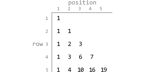
Keyingi asosiy kuzatuv shundaki, biz qiymatlarning o'ziga qiziqmaymiz: faqat har bir sonning pariteti (ya'ni juft yoki toq ekanligiga) qiziqamiz. Bunga ko'ra, uchburchakni 0 juft sonni, 1 esa toq sonni ifodalovchi ikkilik uchburchak sifatida ifodalaб yanada soddalashtirishimiz mumkin:
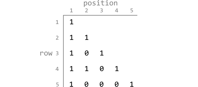
Uchburchakni soddalashtirgandan so'ng, har bir qatordagi birinchi juft sonning pozitsiyalaridagi naqshlarni aniqlash osonlashadi. Buni yanada o'rganaylik.
Naqshlarni aniqlash Juft sonlar faqat 3-qatordan boshlab paydo bo'lganligi sababli 1 va 2-qatorlarni e'tiborsiz qoldiraylik. Naqsh qidirish uchun yaxshi boshlash joyi — har bir qatordagi birinchi juft sonni belgilab, ularning pozitsiyalarini kuzatish:
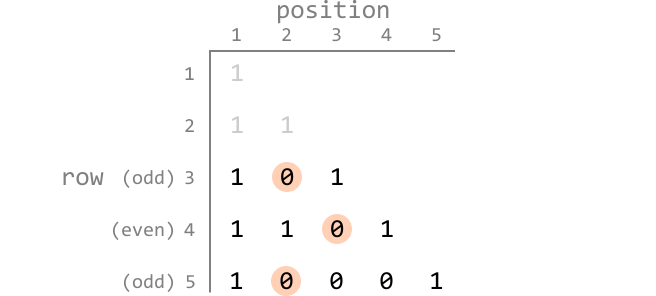
3 dan 5 gacha qatorlardan kuzatilishi mumkin bo'lgan bitta naqsh shundaki, toq raqamli qatorlarda birinchi juft son 2-pozitsiyada. Juft raqamli qatorlarda birinchi juft son 3-pozitsiyada deb ham faraz qilishimiz mumkin.
Bu kuzatuvning izchil ekanligini tasdiqlash uchun yana bir nechta qatorga nazar solaylik:
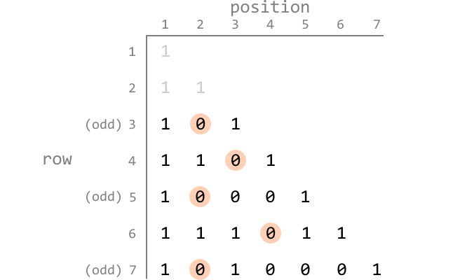
Hozircha toq raqamli qatorlar uchun farazimiz to'g'ri, ammo juft raqamli qatorlar boshqa naqshga ko'rinaяptи. Uni aniqroq belgilash hali qiyin.
Bu naqsh nima ekanligini aniqlash uchun yana bir nechta qatorni ko'rsatishda davom etaylik:
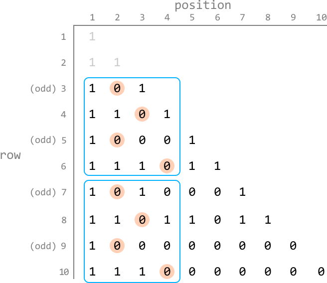
Endi 3 dan 6 gacha qatorlarning birinchi to'rtta ikkilik qiymatining 7 dan 10 gacha qatorlarda takrorlanishini sezamiz. Kelajakdagi qatorlarda davom etsak, bu naqsh takrorlanishda davom etishini payqar edik.
Asosan, quyidagi naqsh 3-qatordan boshlab izchil takrorlanadi:
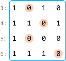
Bu naqsh nima uchun takrorlanishini tushunish uchun qatorning dastlabki to'rtta qiymati faqat oldingi qatorning to'rtta qiymatidan hisoblanishini anglash muhim. Buni uchburchakning boshlang'ich ifodasidan foydalanib quyida vizualizatsiya qilinganini ko'rishimiz mumkin:

Shunday qilib, qatorning boshida ma'lum to'rtta son ketma-ketligi paydo bo'lganda, u keyingi qatorda oldindan aytib bo'ladigan to'rtta son ketma-ketligini yaratadi. Bu kuzatuvni butun naqshga kengaytirib, naqsh bir marta takrorlanganligini (3 dan 6 gacha qatorlardan 7 dan 10 gacha qatorlarga) ko'rib, u cheksiz takrorlanishda davom etishini xulosalashimiz mumkin.
Bu bizga quyidagi davriy mantiqni beradi:
- Agar n toq bo'lsa (n % 2 != 0), 2 ni qaytaring.
- Agar n 4 ning karrali bo'lsa (n % 4 == 0), 3 ni qaytaring.
- Aks holda, 4 ni qaytaring.
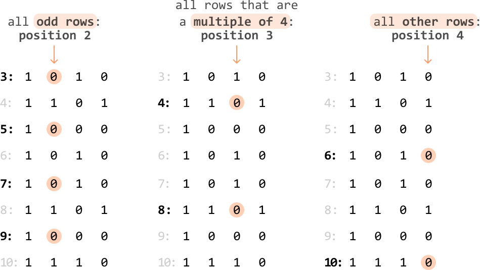
Bu masala naqshlarni tanish va masalani soddalashtirish vaqt sarflaydigan yechimni tez, doimiy vaqtli yechimga aylantirishi mumkinligini ko'rsatadi.
Amalga Oshirish
def triangle_numbers(n: int) -> int:
# If n is an odd-numbered row, the first even number always starts at position
# 2.
if n % 2 != 0:
return 2
# If n is a multiple of 4, the first even number always starts at position 3.
elif n % 4 == 0:
return 3
# For all other rows, the first even number always starts at position 4.
return 4
Murakkablik Tahlili
Vaqt murakkabligi: triangle_numbers ning vaqt murakkabligi O(1).
Xotira murakkabligi: O(1).