Foreword
We are delighted that you have decided to join us in learning the system design interviews. System design interview questions are the most difficult to tackle among all the technical interviews. The questions require the interviewees to design an architecture for a software system, which could be a news feed, Google search, chat system, etc. These questions are intimidating, and there is no certain pattern to follow. The questions are usually very big scoped and vague. The processes are open-ended and unclear without a standard or correct answer.
Companies widely adopt system design interviews because the communication and problem-solving skills tested in these interviews are similar to those required by a software engineer's daily work. An interviewee is evaluated based on how she analyzes a vague problem and how she solves the problem step by step. The abilities tested also involve how she explains the idea, discusses with others, and evaluates and optimizes the system. In English, using "she" flows better than "he or she" or jumping between the two. To make reading easier, we use the feminine pronoun throughout this course. No disrespect is intended for male engineers.
The system design questions are open-ended. Just like in the real world, there are many differences and variations in the system. The desired outcome is to come up with an architecture to achieve system design goals. The discussions could go in different ways depending on the interviewer. Some interviewers may choose high-level architecture to cover all aspects; whereas some might choose one or more areas to focus on. Typically, system requirements, constraints and bottlenecks should be well understood to shape the direction of both the interviewer and interviewee.
The objective of this course is to provide a reliable strategy to approach the system design questions. The right strategy and knowledge are vital to the success of an interview.
This course provides solid knowledge in building a scalable system. The more knowledge gained from reading this course, the better you are equipped in solving the system design questions.
This course also provides a step by step framework on how to tackle a system design question. It provides many examples to illustrate the systematic approach with detailed steps that you can follow. With constant practice, you will be well-equipped to tackle system design interview questions.
Join the Community
We created a members-only Discord group. It is designed for community discussions on the following topics:
- System design fundamentals. - Showcasing design diagrams and getting feedback. - Finding mock interview buddies. - General chat with community members.
Come join us and introduce yourself to the community, today!
Scale From Zero To Millions Of Users
Designing a system that supports millions of users is challenging, and it is a journey that requires continuous refinement and endless improvement. In this chapter, we build a system that supports a single user and gradually scale it up to serve millions of users. After reading this chapter, you will master a handful of techniques that will help you to crack the system design interview questions.
Single server setup
A journey of a thousand miles begins with a single step, and building a complex system is no different. To start with something simple, everything is running on a single server. Figure 1 shows the illustration of a single server setup where everything is running on one server: web app, database, cache, etc.
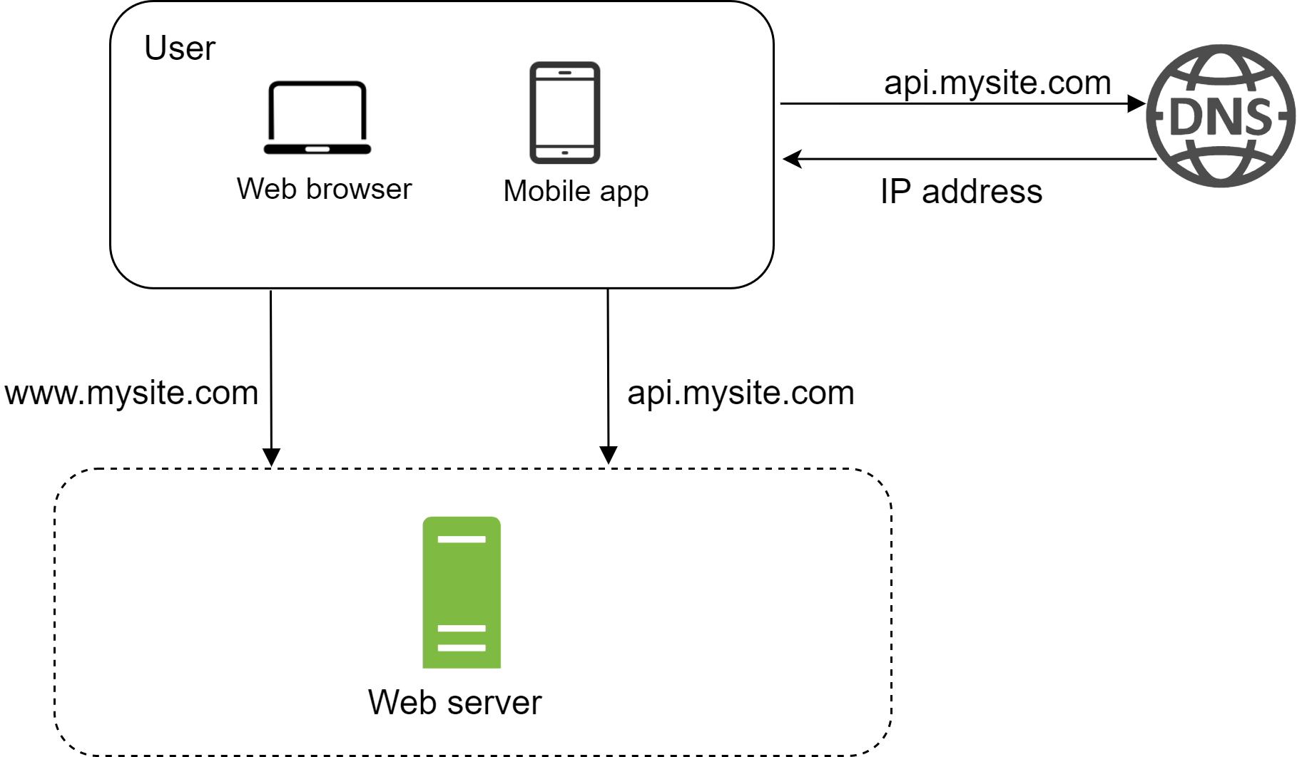
Request flow and traffic source
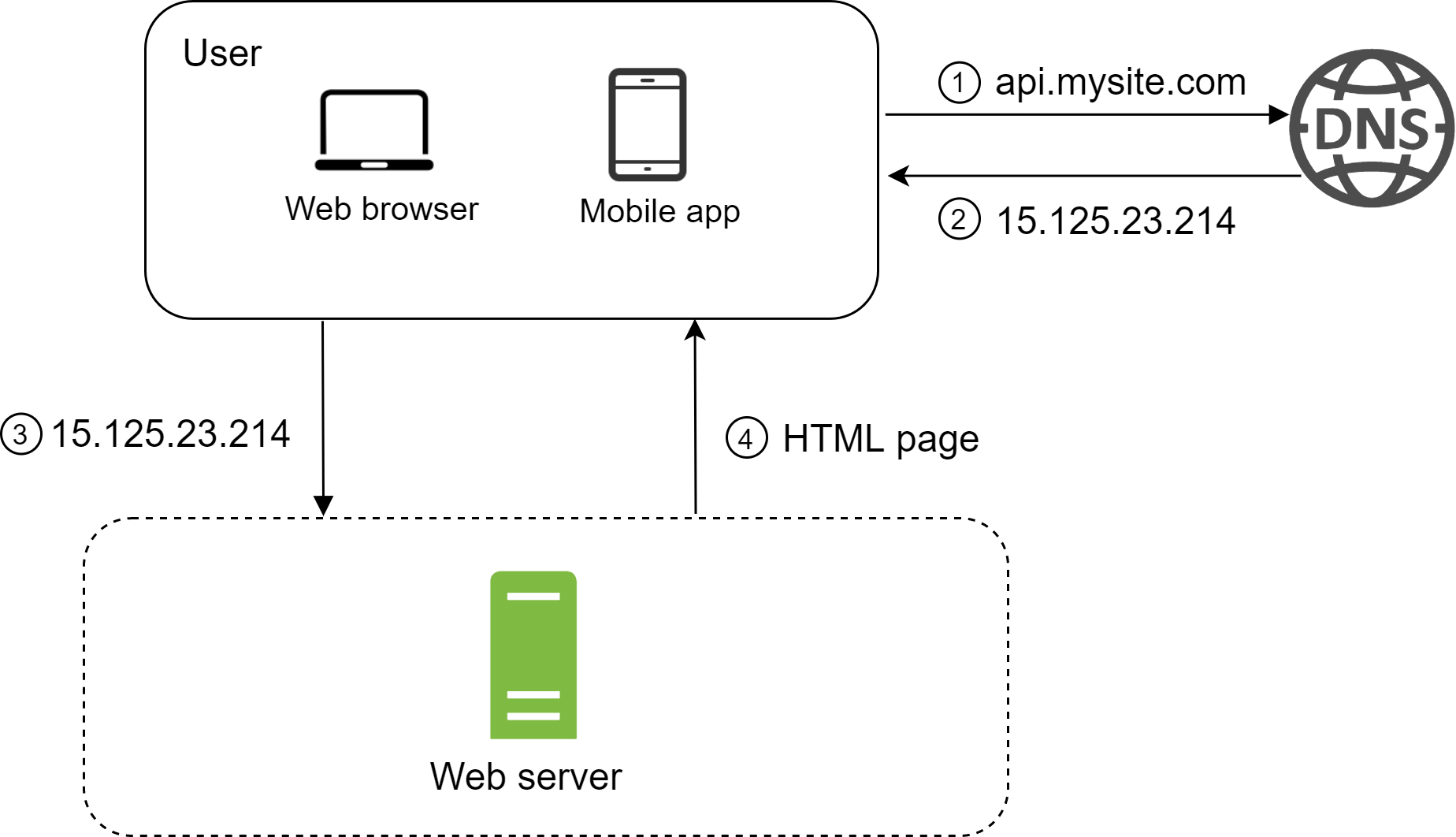
To understand this setup, it is helpful to investigate the request flow and traffic source. Let us first look at the request flow (Figure 2).
1. Users access websites through domain names, such as api.mysite.com. Usually, the Domain Name System (DNS) is a paid service provided by 3rd parties and not hosted by our servers.
2. Internet Protocol (IP) address is returned to the browser or mobile app. In the example, IP address 15.125.23.214 is returned.
3. Once the IP address is obtained, Hypertext Transfer Protocol (HTTP) [1] requests are sent directly to your web server.
4. The web server returns HTML pages or JSON response for rendering.
Next, let us examine the traffic source. The traffic to your web server comes from two sources: web application and mobile application.
**Web application:** it uses a combination of server-side languages (Java, Python, etc.) to handle business logic, storage, etc., and client-side languages (HTML and JavaScript) for presentation.
**Mobile application:** HTTP protocol is the communication protocol between the mobile app and the web server. JavaScript Object Notation (JSON) is commonly used API response format to transfer data due to its simplicity. An example of the API response in JSON format is shown below:
``` GET /users/12 – Retrieve user object for id = 12
{ "id": 12, "firstName": "John", "lastName": "Smith", "address": { "streetAddress": "21 2nd Street", "city": "New York", "state": "NY", "postalCode": 10021 }, "phoneNumbers": [ "212 555-1234", "646 555-4567" ] } ```
Database
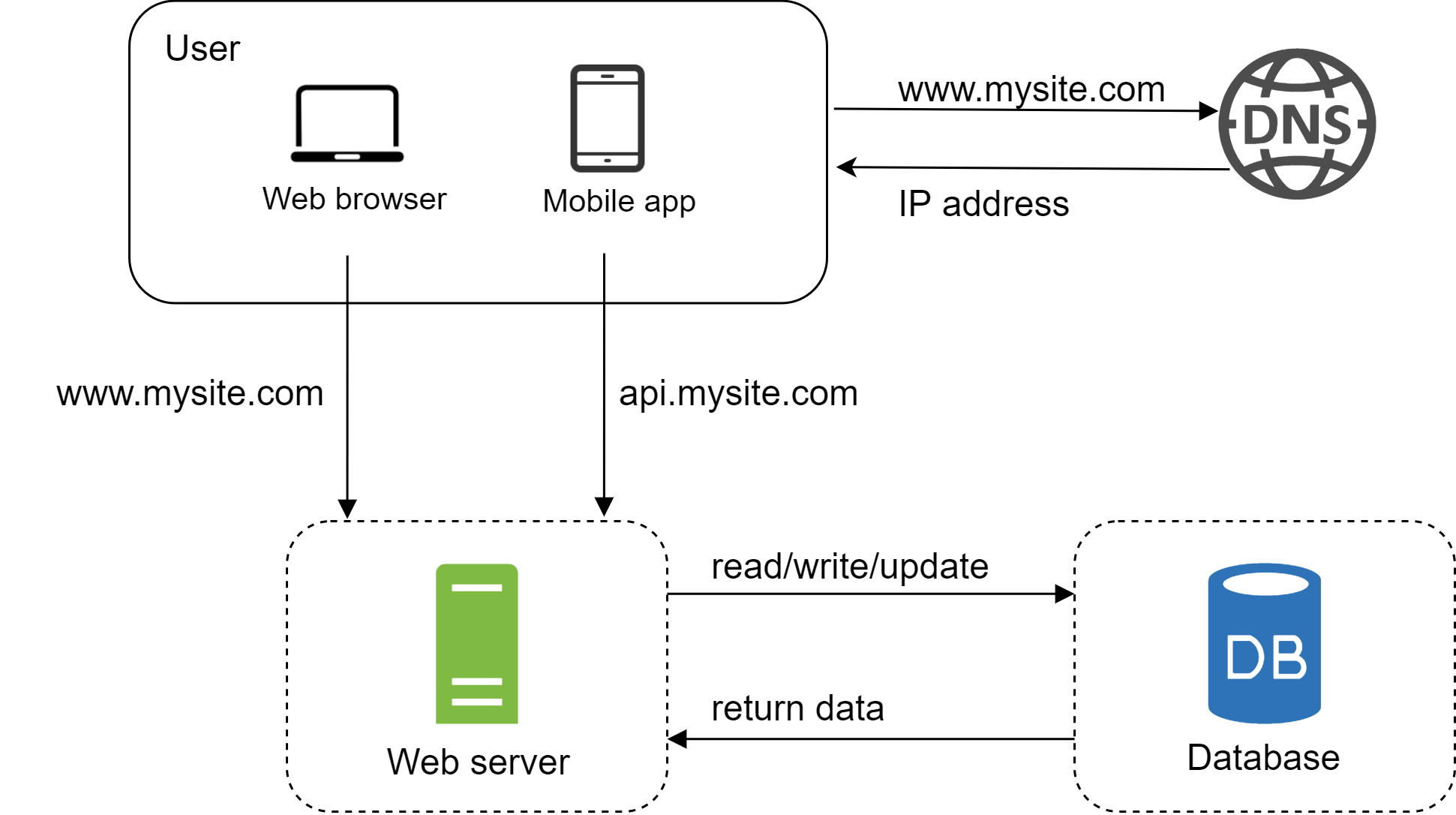
With the growth of the user base, one server is not enough, and we need multiple servers: one for web/mobile traffic, the other for the database (Figure 3). Separating web/mobile traffic (web tier) and database (data tier) servers allows them to be scaled independently.
Which databases to use?
You can choose between a traditional relational database and a non-relational database. Let us examine their differences.
**Relational databases** are also called a relational database management system (RDBMS) or SQL database. The most popular ones are MySQL, Oracle database, PostgreSQL, etc. Relational databases represent and store data in tables and rows. You can perform join operations using SQL across different database tables.
**Non-Relational databases** are also called NoSQL databases. Popular ones are CouchDB, Neo4j, Cassandra, HBase, Amazon DynamoDB, etc. [2]. These databases are grouped into four categories: key-value stores, graph stores, column stores, and document stores. Join operations are generally not supported in non-relational databases.
For most developers, relational databases are the best option because they have been around for over 40 years and historically, they have worked well. However, if relational databases are not suitable for your specific use cases, it is critical to explore beyond relational databases. Non-relational databases might be the right choice if:
- Your application requires super-low latency. - Your data are unstructured, or you do not have any relational data. - You only need to serialize and deserialize data (JSON, XML, YAML, etc.). - You need to store a massive amount of data.
Vertical scaling vs horizontal scaling
Vertical scaling, referred to as "scale up", means the process of adding more power (CPU, RAM, etc.) to your servers. Horizontal scaling, referred to as "scale-out", allows you to scale by adding more servers into your pool of resources.
When traffic is low, vertical scaling is a great option, and the simplicity of vertical scaling is its main advantage. Unfortunately, it comes with serious limitations:
- Vertical scaling has a hard limit. It is impossible to add unlimited CPU and memory to a single server. - Vertical scaling does not have failover and redundancy. If one server goes down, the website/app goes down with it completely.
Horizontal scaling is more desirable for large scale applications due to the limitations of vertical scaling.
In the previous design, users are connected to the web server directly. Users will unable to access the website if the web server is offline. In another scenario, if many users access the web server simultaneously and it reaches the web server's load limit, users generally experience slower response or fail to connect to the server. A load balancer is the best technique to address these problems.
Load balancer
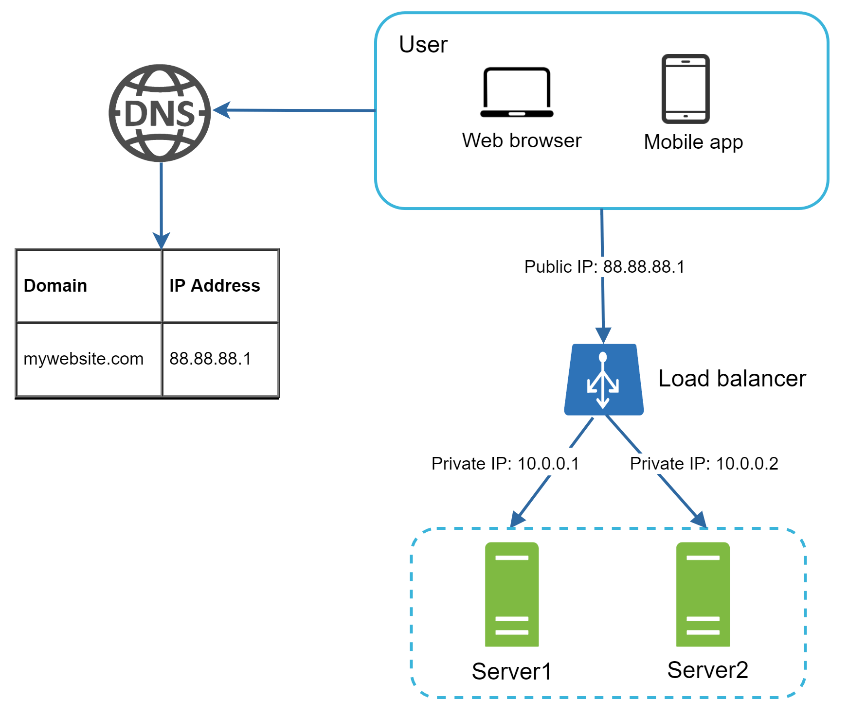
A load balancer evenly distributes incoming traffic among web servers that are defined in a load-balanced set. Figure 4 shows how a load balancer works.
As shown in Figure 4, users connect to the public IP of the load balancer directly. With this setup, web servers are unreachable directly by clients anymore. For better security, private IPs are used for communication between servers. A private IP is an IP address reachable only between servers in the same network; however, it is unreachable over the internet. The load balancer communicates with web servers through private IPs.
In Figure 4, after a load balancer and a second web server are added, we successfully solved no failover issue and improved the availability of the web tier. Details are explained below:
- If server 1 goes offline, all the traffic will be routed to server 2. This prevents the website from going offline. We will also add a new healthy web server to the server pool to balance the load. - If the website traffic grows rapidly, and two servers are not enough to handle the traffic, the load balancer can handle this problem gracefully. You only need to add more servers to the web server pool, and the load balancer automatically starts to send requests to them.
Now the web tier looks good, what about the data tier? The current design has one database, so it does not support failover and redundancy. Database replication is a common technique to address those problems.
Database replication
Quoted from Wikipedia: "Database replication can be used in many database management systems, usually with a master/slave relationship between the original (master) and the copies (slaves)" [3].
A master database generally only supports write operations. A slave database gets copies of the data from the master database and only supports read operations. All the data-modifying commands like insert, delete, or update must be sent to the master database. Most applications require a much higher ratio of reads to writes; thus, the number of slave databases in a system is usually larger than the number of master databases. Figure 5 shows a master database with multiple slave databases.
**Advantages of database replication:**
- **Better performance:** In the master-slave model, all writes and updates happen in master nodes; whereas, read operations are distributed across slave nodes. This model improves performance because it allows more queries to be processed in parallel. - **Reliability:** If one of your database servers is destroyed by a natural disaster, such as a typhoon or an earthquake, data is still preserved. You do not need to worry about data loss because data is replicated across multiple locations. - **High availability:** By replicating data across different locations, your website remains in operation even if a database is offline as you can access data stored in another database server.
In the previous section, we discussed how a load balancer helped to improve system availability. We ask the same question here: what if one of the databases goes offline?
- If only one slave database is available and it goes offline, read operations will be directed to the master database temporarily. As soon as the issue is found, a new slave database will replace the old one. In case multiple slave databases are available, read operations are redirected to other healthy slave databases. A new database server will replace the old one. - If the master database goes offline, a slave database will be promoted to be the new master. All the database operations will be temporarily executed on the new master database. A new slave database will replace the old one for data replication immediately. In production systems, promoting a new master is more complicated as the data in a slave database might not be up to date. The missing data needs to be updated by running data recovery scripts. Although some other replication methods like multi-masters and circular replication could help, those setups are more complicated; and their discussions are beyond the scope of this course. Interested readers should refer to the listed reference materials [4] [5].
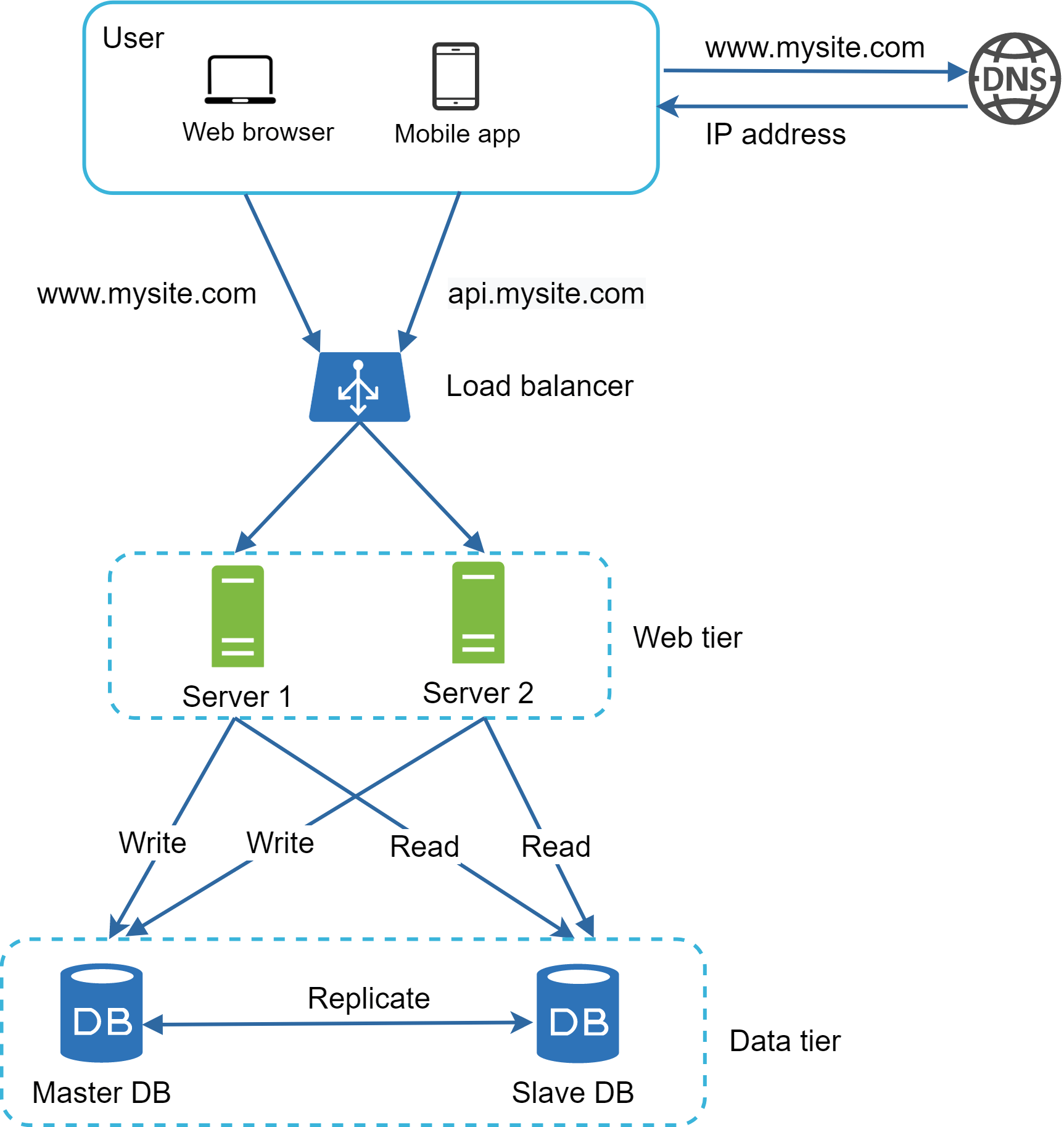
Figure 6 shows the system design after adding the load balancer and database replication.
Let us take a look at the design: - A user gets the IP address of the load balancer from DNS. - A user connects the load balancer with this IP address. - The HTTP request is routed to either Server 1 or Server 2. - A web server reads user data from a slave database. - A web server routes any data-modifying operations to the master database. This includes write, update, and delete operations.

Cache
A cache is a temporary storage area that stores the result of expensive responses or frequently accessed data in memory so that subsequent requests are served more quickly. As illustrated in Figure 6, every time a new web page loads, one or more database calls are executed to fetch data. The application performance is greatly affected by calling the database repeatedly. The cache can mitigate this problem.
Cache tier
The cache tier is a temporary data store layer, much faster than the database. The benefits of having a separate cache tier include better system performance, ability to reduce database workloads, and the ability to scale the cache tier independently. Figure 7 shows a possible setup of a cache server.
After receiving a request, a web server first checks if the cache has the available response. If it has, it sends data back to the client. If not, it queries the database, stores the response in cache, and sends it back to the client. This caching strategy is called a read-through cache. Other caching strategies are available depending on the data type, size, and access patterns. A previous study explains how different caching strategies work [6].
Interacting with cache servers is simple because most cache servers provide APIs for common programming languages. The following code snippet shows typical Memcached APIs:
``` SECONDS = 1 cache.set('myKey', 'hi there', 3600 * SECONDS) cache.get('myKey') ```

Considerations for using cache
Here are a few considerations for using a cache system:
- **Decide when to use cache.** Consider using cache when data is read frequently but modified infrequently. Since cached data is stored in volatile memory, a cache server is not ideal for persisting data. For instance, if a cache server restarts, all the data in memory is lost. Thus, important data should be saved in persistent data stores.
- **Expiration policy.** It is a good practice to implement an expiration policy. Once cached data is expired, it is removed from the cache. When there is no expiration policy, cached data will be stored in the memory permanently. It is advisable not to make the expiration date too short as this will cause the system to reload data from the database too frequently. Meanwhile, it is advisable not to make the expiration date too long as the data can become stale.
- **Consistency:** This involves keeping the data store and the cache in sync. Inconsistency can happen because data-modifying operations on the data store and cache are not in a single transaction. When scaling across multiple regions, maintaining consistency between the data store and cache is challenging. For further details, refer to the paper titled "Scaling Memcache at Facebook" published by Facebook [7].
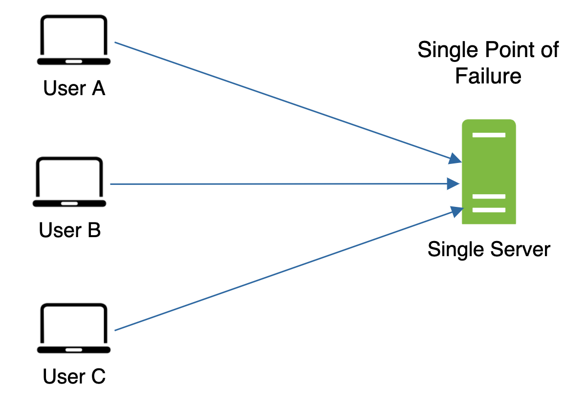
- **Mitigating failures:** A single cache server represents a potential single point of failure (SPOF), defined in Wikipedia as follows: "A single point of failure (SPOF) is a part of a system that, if it fails, will stop the entire system from working" [8]. As a result, multiple cache servers across different data centers are recommended to avoid SPOF. Another recommended approach is to overprovision the required memory by certain percentages. This provides a buffer as the memory usage increases.
- **Eviction Policy:** Once the cache is full, any requests to add items to the cache might cause existing items to be removed. This is called cache eviction. Least-recently-used (LRU) is the most popular cache eviction policy. Other eviction policies, such as the Least Frequently Used (LFU) or First in First Out (FIFO), can be adopted to satisfy different use cases.
Content delivery network (CDN)
A CDN is a network of geographically dispersed servers used to deliver static content. CDN servers cache static content like images, videos, CSS, JavaScript files, etc.
Dynamic content caching is a relatively new concept and beyond the scope of this course. It enables the caching of HTML pages that are based on request path, query strings, cookies, and request headers. Refer to the article mentioned in reference material [9] for more about this. This course focuses on how to use CDN to cache static content.
Here is how CDN works at the high-level: when a user visits a website, a CDN server closest to the user will deliver static content. Intuitively, the further users are from CDN servers, the slower the website loads. For example, if CDN servers are in San Francisco, users in Los Angeles will get content faster than users in Europe. Figure 9 is a great example that shows how CDN improves load time.
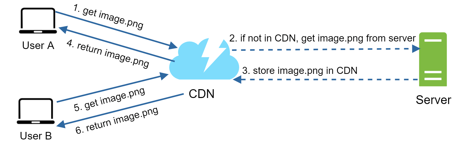
Figure 10 demonstrates the CDN workflow:
1. User A tries to get image.png by using an image URL. The URL's domain is provided by the CDN provider. The following two image URLs are samples used to demonstrate what image URLs look like on Amazon and Akamai CDNs: - `https://mysite.cloudfront.net/logo.jpg` - `https://mysite.akamai.com/image-manager/img/logo.jpg`
2. If the CDN server does not have image.png in the cache, the CDN server requests the file from the origin, which can be a web server or online storage like Amazon S3.
3. The origin returns image.png to the CDN server, which includes optional HTTP header Time-to-Live (TTL) which describes how long the image is cached.
4. The CDN caches the image and returns it to User A. The image remains cached in the CDN until the TTL expires.
5. User B sends a request to get the same image.
6. The image is returned from the cache as long as the TTL has not expired.

Considerations of using a CDN
- **Cost:** CDNs are run by third-party providers, and you are charged for data transfers in and out of the CDN. Caching infrequently used assets provides no significant benefits so you should consider moving them out of the CDN.
- **Setting an appropriate cache expiry:** For time-sensitive content, setting a cache expiry time is important. The cache expiry time should neither be too long nor too short. If it is too long, the content might no longer be fresh. If it is too short, it can cause repeat reloading of content from origin servers to the CDN.
- **CDN fallback:** You should consider how your website/application copes with CDN failure. If there is a temporary CDN outage, clients should be able to detect the problem and request resources from the origin.
- **Invalidating files:** You can remove a file from the CDN before it expires by performing one of the following operations: - Invalidate the CDN object using APIs provided by CDN vendors. - Use object versioning to serve a different version of the object. To version an object, you can add a parameter to the URL, such as a version number. For example, version number 2 is added to the query string: `image.png?v=2`.
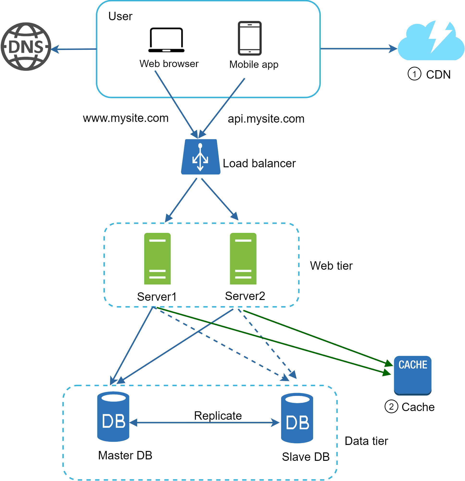
Figure 11 shows the design after the CDN and cache are added: 1. Static assets (JS, CSS, images, etc.) are no longer served by web servers. They are fetched from the CDN for better performance. 2. The database load is lightened by caching data.
Stateless web tier
Now it is time to consider scaling the web tier horizontally. For this, we need to move state (for instance user session data) out of the web tier. A good practice is to store session data in the persistent storage such as relational database or NoSQL. Each web server in the cluster can access state data from databases. This is called stateless web tier.
Stateful architecture
A stateful server and stateless server has some key differences. A stateful server remembers client data (state) from one request to the next. A stateless server keeps no state information.
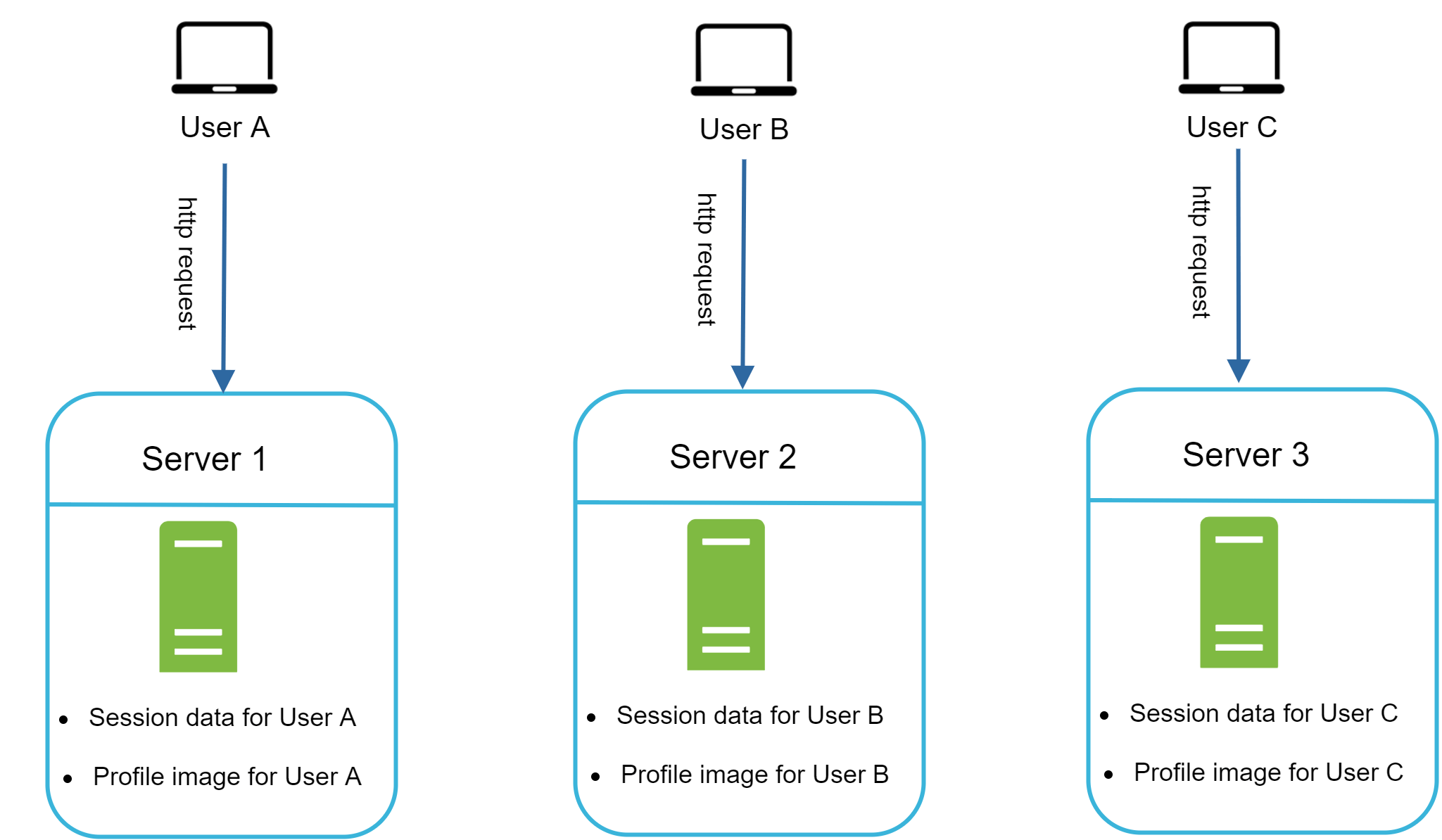
Figure 12 shows an example of a stateful architecture.
In Figure 12, user A's session data and profile image are stored in Server 1. To authenticate User A, HTTP requests must be routed to Server 1. If a request is sent to other servers like Server 2, authentication would fail because Server 2 does not contain User A's session data. Similarly, all HTTP requests from User B must be routed to Server 2; all requests from User C must be sent to Server 3.
The issue is that every request from the same client must be routed to the same server. This can be done with sticky sessions in most load balancers [10]; however, this adds the overhead. Adding or removing servers is much more difficult with this approach. It is also challenging to handle server failures.
Stateless architecture
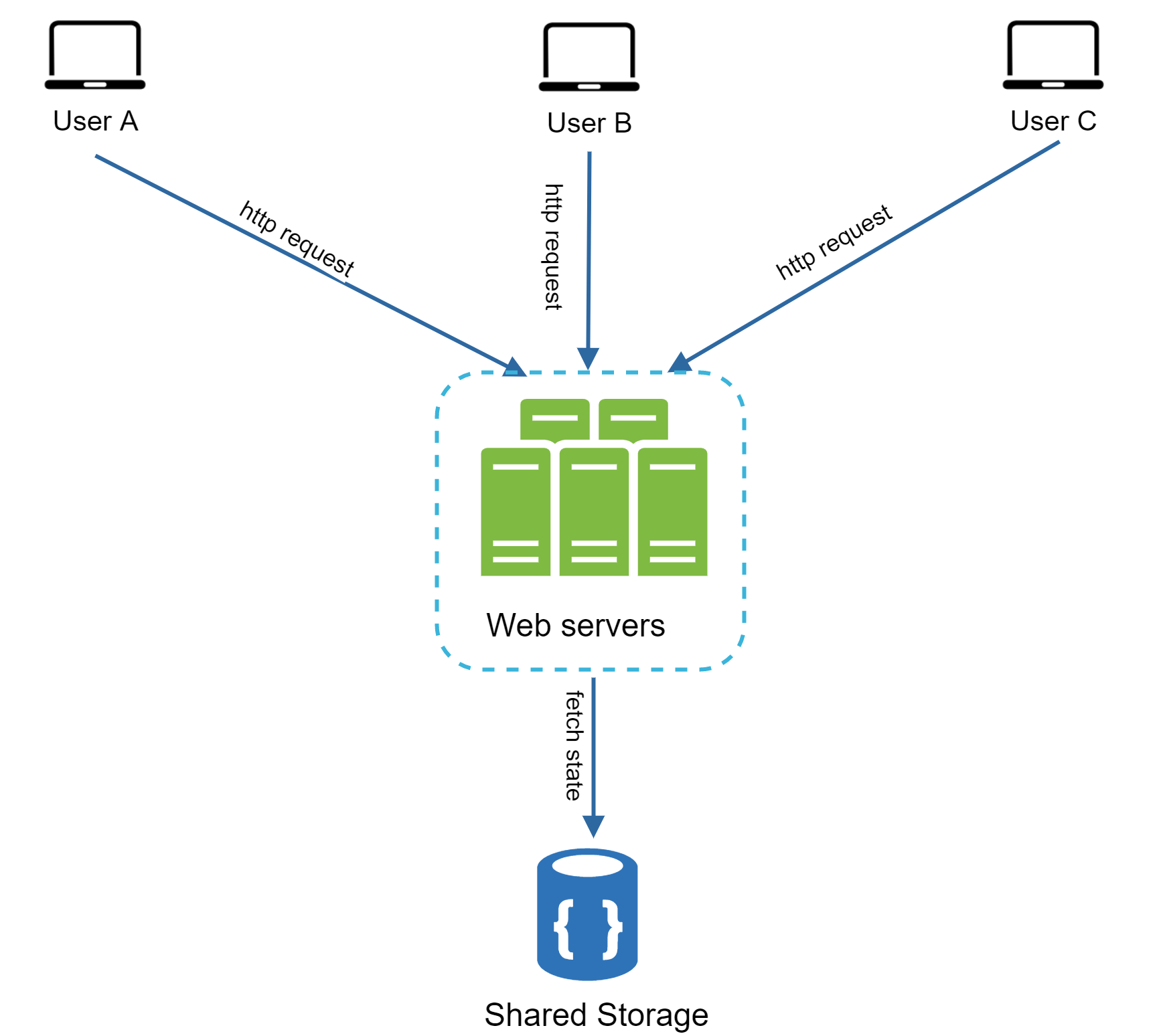
Figure 13 shows the stateless architecture.
In this stateless architecture, HTTP requests from users can be sent to any web servers, which fetch state data from a shared data store. State data is stored in a shared data store and kept out of web servers. A stateless system is simpler, more robust, and scalable.
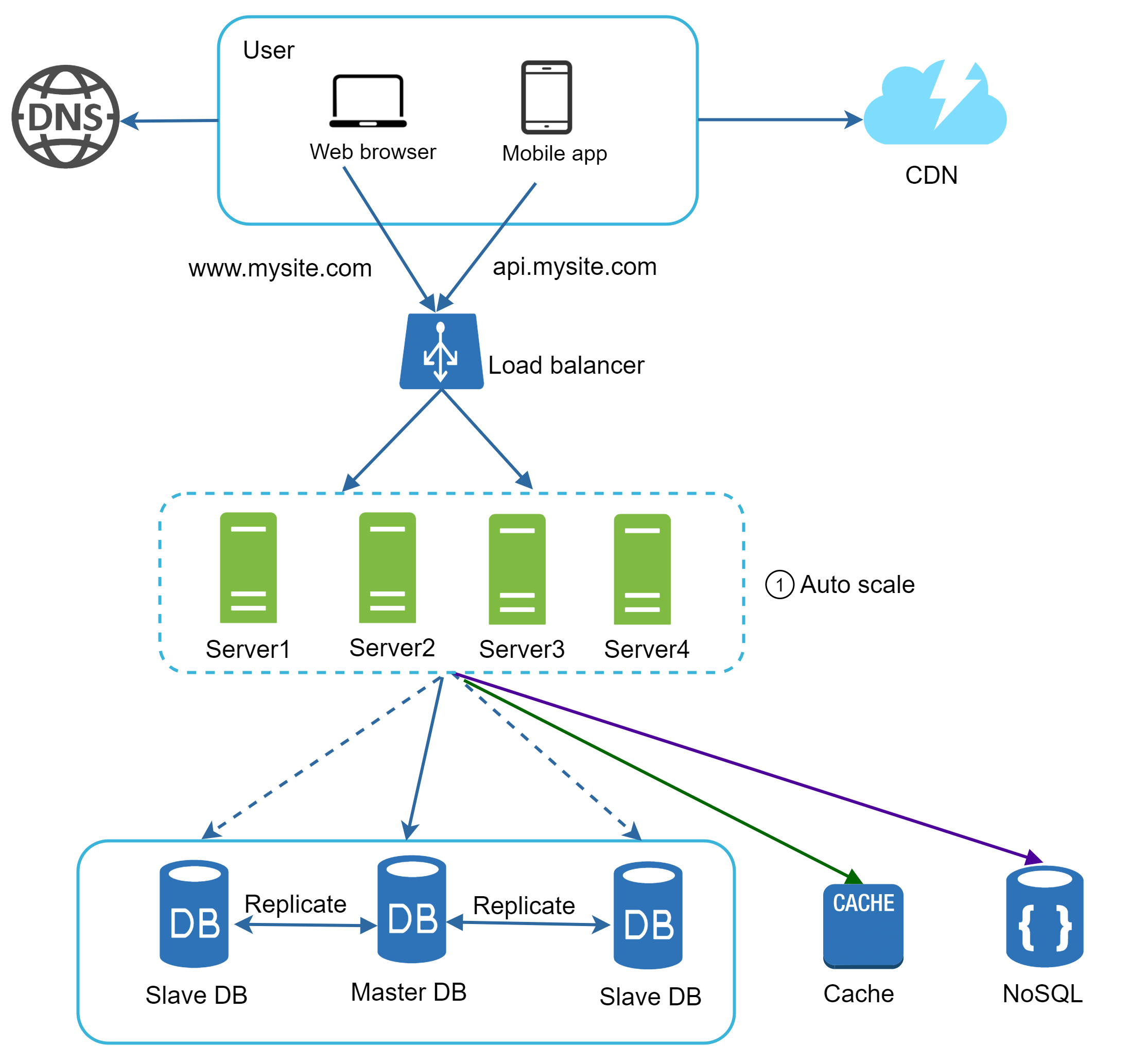
Figure 14 shows the updated design with a stateless web tier.
In Figure 14, we move the session data out of the web tier and store them in the persistent data store. The shared data store could be a relational database, Memcached/Redis, NoSQL, etc. The NoSQL data store is chosen as it is easy to scale. Autoscaling means adding or removing web servers automatically based on the traffic load. After the state data is removed out of web servers, auto-scaling of the web tier is easily achieved by adding or removing servers based on traffic load.
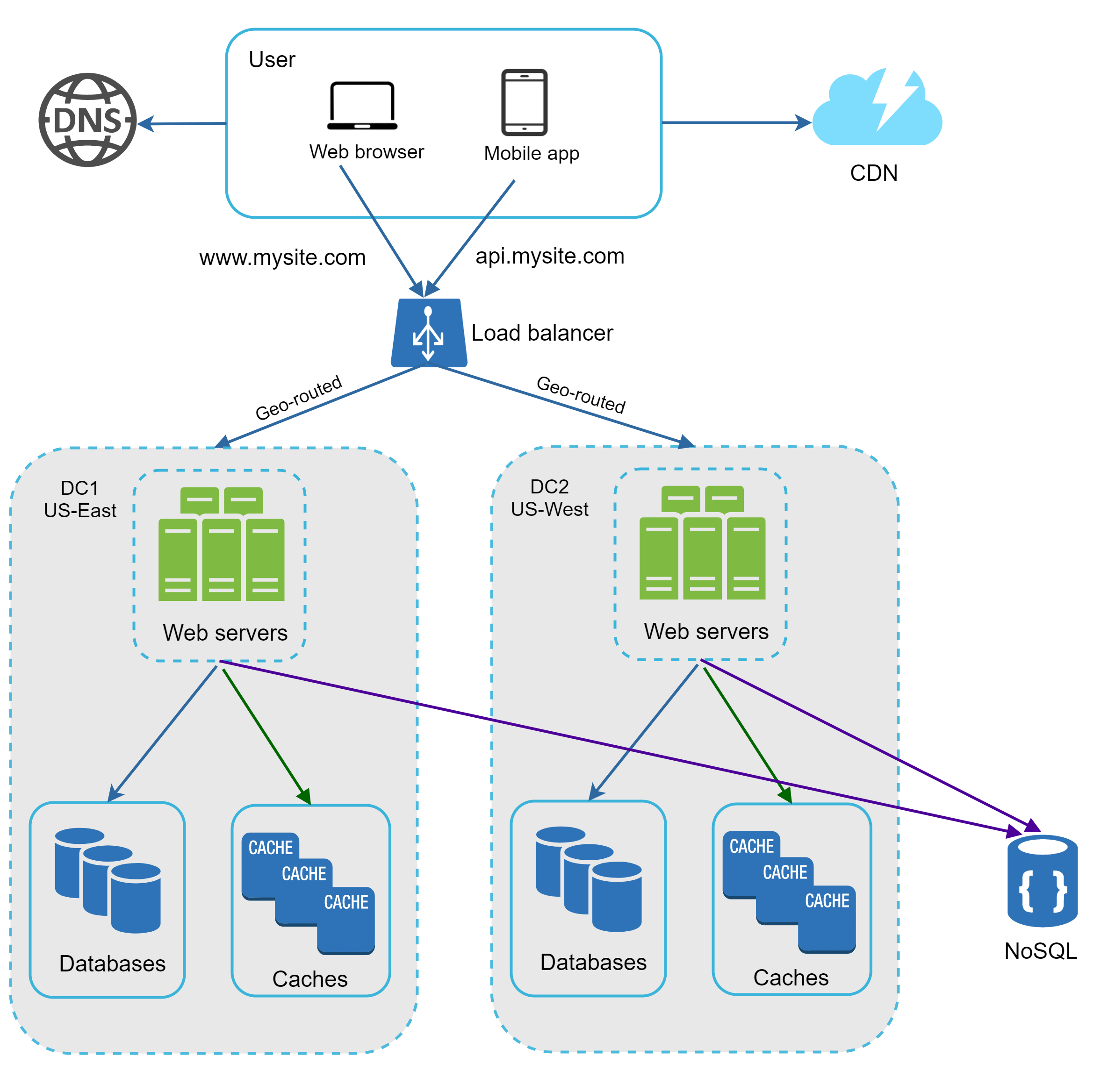
Your website grows rapidly and attracts a significant number of users internationally. To improve availability and provide a better user experience across wider geographical areas, supporting multiple data centers is crucial.
Data centers
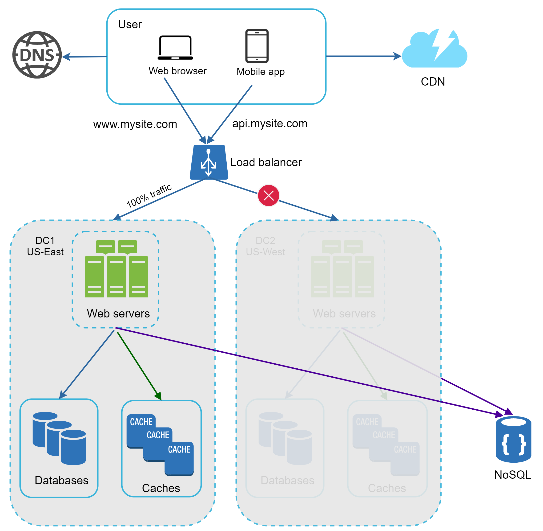
Figure 15 shows an example setup with two data centers. In normal operation, users are geoDNS-routed, also known as geo-routed, to the closest data center, with a split traffic of x% in US-East and (100 – x)% in US-West. geoDNS is a DNS service that allows domain names to be resolved to IP addresses based on the location of a user.
In the event of any significant data center outage, we direct all traffic to a healthy data center. In Figure 16, data center 2 (US-West) is offline, and 100% of the traffic is routed to data center 1 (US-East).
Several technical challenges must be resolved to achieve multi-data center setup:
- **Traffic redirection:** Effective tools are needed to direct traffic to the correct data center. GeoDNS can be used to direct traffic to the nearest data center depending on where a user is located.
- **Data synchronization:** Users from different regions could use different local databases or caches. In failover cases, traffic might be routed to a data center where data is unavailable. A common strategy is to replicate data across multiple data centers. A previous study shows how Netflix implements asynchronous multi-data center replication [11].
- **Test and deployment:** With multi-data center setup, it is important to test your website/application at different locations. Automated deployment tools are vital to keep services consistent through all the data centers [11].
To further scale our system, we need to decouple different components of the system so they can be scaled independently. Messaging queue is a key strategy employed by many real-world distributed systems to solve this problem.
Message queue
A message queue is a durable component, stored in memory, that supports asynchronous communication. It serves as a buffer and distributes asynchronous requests. The basic architecture of a message queue is simple. Input services, called producers/publishers, create messages, and publish them to a message queue. Other services or servers, called consumers/subscribers, connect to the queue, and perform actions defined by the messages. The model is shown in Figure 17.
Decoupling makes the message queue a preferred architecture for building a scalable and reliable application. With the message queue, the producer can post a message to the queue when the consumer is unavailable to process it. The consumer can read messages from the queue even when the producer is unavailable.
Consider the following use case: your application supports photo customization, including cropping, sharpening, blurring, etc. Those customization tasks take time to complete. In Figure 18, web servers publish photo processing jobs to the message queue. Photo processing workers pick up jobs from the message queue and asynchronously perform photo customization tasks. The producer and the consumer can be scaled independently. When the size of the queue becomes large, more workers are added to reduce the processing time. However, if the queue is empty most of the time, the number of workers can be reduced.


Logging, metrics, automation
When working with a small website that runs on a few servers, logging, metrics, and automation support are good practices but not a necessity. However, now that your site has grown to serve a large business, investing in those tools is essential.
- **Logging:** Monitoring error logs is important because it helps to identify errors and problems in the system. You can monitor error logs at per server level or use tools to aggregate them to a centralized service for easy search and viewing.
- **Metrics:** Collecting different types of metrics help us to gain business insights and understand the health status of the system. Some of the following metrics are useful: - Host level metrics: CPU, Memory, disk I/O, etc. - Aggregated level metrics: for example, the performance of the entire database tier, cache tier, etc. - Key business metrics: daily active users, retention, revenue, etc.
- **Automation:** When a system gets big and complex, we need to build or leverage automation tools to improve productivity. Continuous integration is a good practice, in which each code check-in is verified through automation, allowing teams to detect problems early. Besides, automating your build, test, deploy process, etc. could improve developer productivity significantly.
Adding message queues and different tools
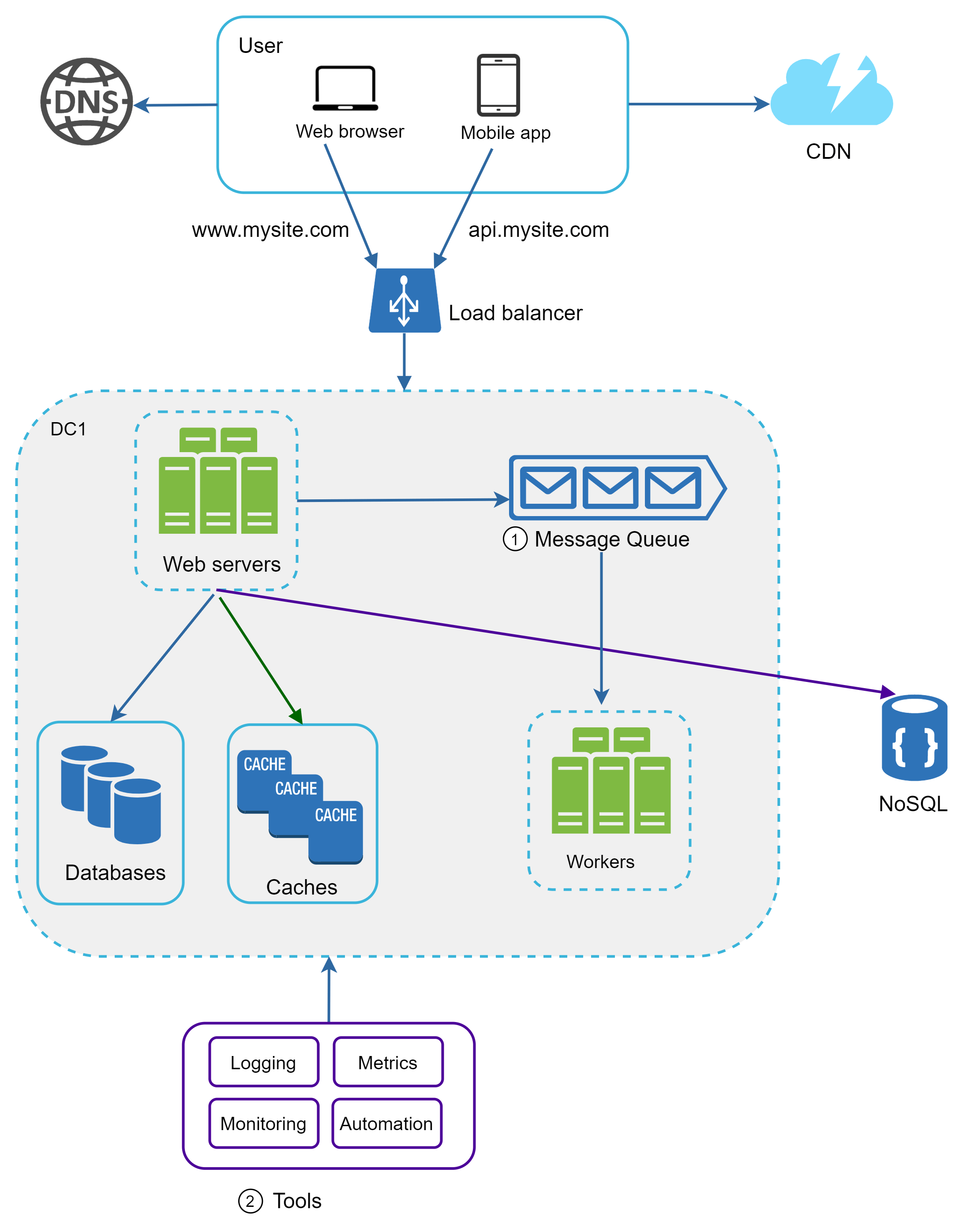
Figure 19 shows the updated design. Due to the space constraint, only one data center is shown in the figure.
1. The design includes a message queue, which helps to make the system more loosely coupled and failure resilient. 2. Logging, monitoring, metrics, and automation tools are included.
As the data grows every day, your database gets more overloaded. It is time to scale the data tier.
Database scaling
There are two broad approaches for database scaling: vertical scaling and horizontal scaling.
Vertical scaling
Vertical scaling, also known as scaling up, is the scaling by adding more power (CPU, RAM, DISK, etc.) to an existing machine. There are some powerful database servers. According to Amazon Relational Database Service (RDS) [12], you can get a database server with 24 TB of RAM. This kind of powerful database server could store and handle lots of data. For example, stackoverflow.com in 2013 had over 10 million monthly unique visitors, but it only had 1 master database [13]. However, vertical scaling comes with some serious drawbacks:
- You can add more CPU, RAM, etc. to your database server, but there are hardware limits. If you have a large user base, a single server is not enough. - Greater risk of single point of failures. - The overall cost of vertical scaling is high. Powerful servers are much more expensive.
Horizontal scaling
Horizontal scaling, also known as sharding, is the practice of adding more servers. Figure 20 compares vertical scaling with horizontal scaling.
Sharding separates large databases into smaller, more easily managed parts called shards. Each shard shares the same schema, though the actual data on each shard is unique to the shard.
Figure 21 shows an example of sharded databases. User data is allocated to a database server based on user IDs. Anytime you access data, a hash function is used to find the corresponding shard. In our example, user_id % 4 is used as the hash function. If the result equals to 0, shard 0 is used to store and fetch data. If the result equals to 1, shard 1 is used. The same logic applies to other shards.
Figure 22 shows the user table in sharded databases.
The most important factor to consider when implementing a sharding strategy is the choice of the sharding key. Sharding key (known as a partition key) consists of one or more columns that determine how data is distributed. As shown in Figure 22, "user_id" is the sharding key. A sharding key allows you to retrieve and modify data efficiently by routing database queries to the correct database. When choosing a sharding key, one of the most important criteria is to choose a key that can evenly distributed data.
Sharding is a great technique to scale the database but it is far from a perfect solution. It introduces complexities and new challenges to the system:
- **Resharding data:** Resharding data is needed when 1) a single shard could no longer hold more data due to rapid growth. 2) Certain shards might experience shard exhaustion faster than others due to uneven data distribution. When shard exhaustion happens, it requires updating the sharding function and moving data around. Consistent hashing is a commonly used technique to solve this problem.
- **Celebrity problem:** This is also called a hotspot key problem. Excessive access to a specific shard could cause server overload. Imagine data for Katy Perry, Justin Bieber, and Lady Gaga all end up on the same shard. For social applications, that shard will be overwhelmed with read operations. To solve this problem, we may need to allocate a shard for each celebrity. Each shard might even require further partition.
- **Join and de-normalization:** Once a database has been sharded across multiple servers, it is hard to perform join operations across database shards. A common workaround is to de-normalize the database so that queries can be performed in a single table.
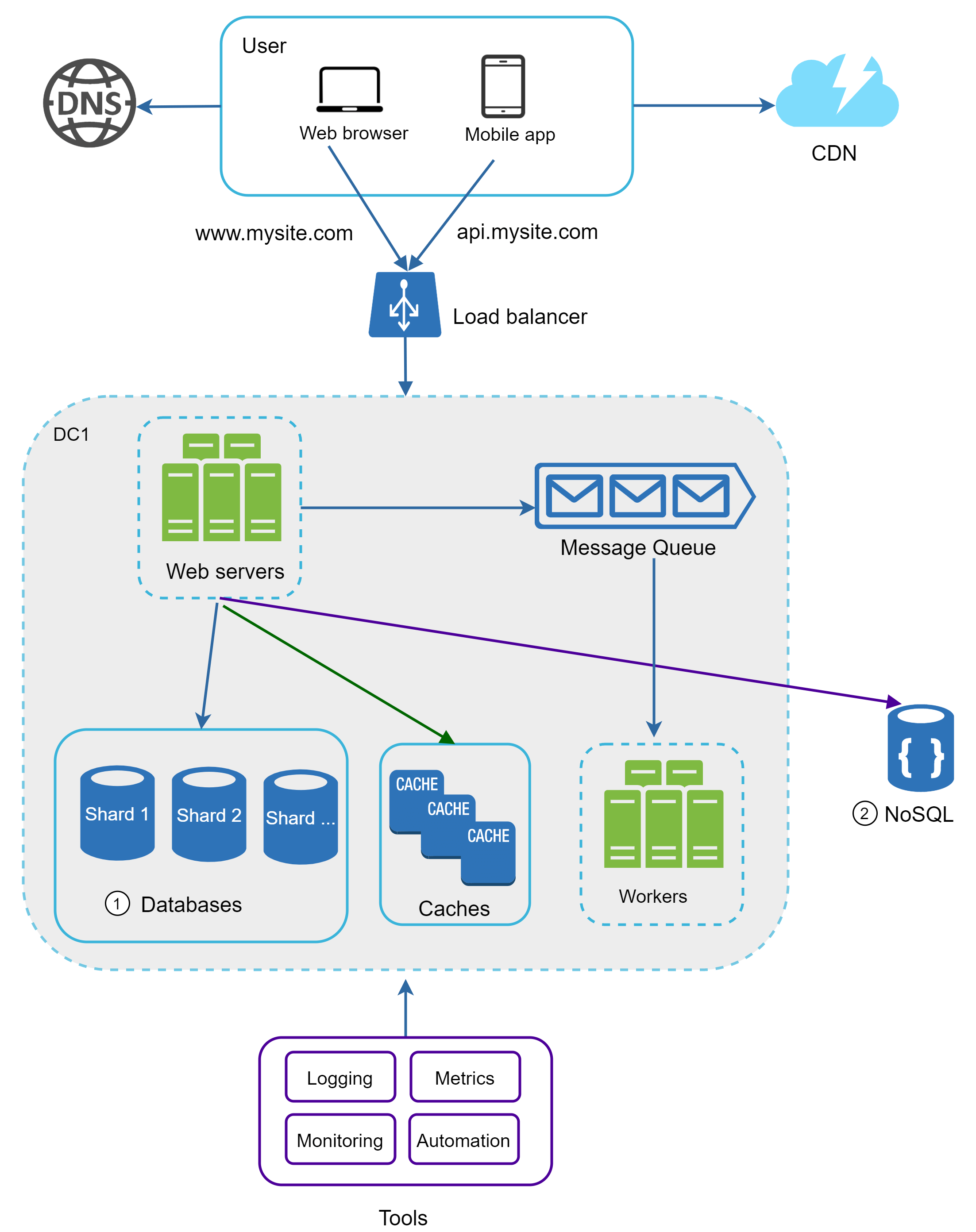
In Figure 23, we shard databases to support rapidly increasing data traffic. At the same time, some of the non-relational functionalities are moved to a NoSQL data store to reduce the database load. Here is an article that covers many use cases of NoSQL [14].


Millions of users and beyond
Scaling a system is an iterative process. Iterating on what we have learned in this chapter could get us far. More fine-tuning and new strategies are needed to scale beyond millions of users. For example, you might need to optimize your system and decouple the system to even smaller services. All the techniques learned in this chapter should provide a good foundation to tackle new challenges. To conclude this chapter, we provide a summary of how we scale our system to support millions of users:
- Keep web tier stateless - Build redundancy at every tier - Cache data as much as you can - Support multiple data centers - Host static assets in CDN - Scale your data tier by sharding - Split tiers into individual services - Monitor your system and use automation tools
Congratulations on getting this far! Now give yourself a pat on the back. Good job!
Back-of-the-envelope Estimation
In a system design interview, sometimes you are asked to estimate system capacity or performance requirements using a back-of-the-envelope estimation. According to Jeff Dean, Google Senior Fellow, "back-of-the-envelope calculations are estimates you create using a combination of thought experiments and common performance numbers to get a good feel for which designs will meet your requirements" [1].
You need to have a good sense of scalability basics to effectively carry out back-of-the-envelope estimation. The following concepts should be well understood: power of two [2], latency numbers every programmer should know, and availability numbers.
Power of two
Although data volume can become enormous when dealing with distributed systems, calculation all boils down to the basics. To obtain correct calculations, it is critical to know the data volume unit using the power of 2. A byte is a sequence of 8 bits. An ASCII character uses one byte of memory (8 bits). Below is a table explaining the data volume unit.
| Power | Approximate value | Full name | Short name | |-------|-------------------|-----------|------------| | 10 | 1 Thousand | 1 Kilobyte | 1 KB | | 20 | 1 Million | 1 Megabyte | 1 MB | | 30 | 1 Billion | 1 Gigabyte | 1 GB | | 40 | 1 Trillion | 1 Terabyte | 1 TB | | 50 | 1 Quadrillion | 1 Petabyte | 1 PB |
**Table 1: Data volume units (powers of 2)**
Latency numbers every programmer should know
Dr. Dean from Google reveals the length of typical computer operations in 2010 [1]. Some numbers are outdated as computers become faster and more powerful. However, those numbers should still be able to give us an idea of the fastness and slowness of different computer operations.
| Operation name | Time | |----------------|------| | L1 cache reference | 0.5 ns | | Branch mispredict | 5 ns | | L2 cache reference | 7 ns | | Mutex lock/unlock | 100 ns | | Main memory reference | 100 ns | | Compress 1K bytes with Zippy | 10,000 ns = 10 µs | | Send 2K bytes over 1 Gbps network | 20,000 ns = 20 µs | | Read 1 MB sequentially from memory | 250,000 ns = 250 µs | | Round trip within the same datacenter | 500,000 ns = 500 µs | | Disk seek | 10,000,000 ns = 10 ms | | Read 1 MB sequentially from the network | 10,000,000 ns = 10 ms | | Read 1 MB sequentially from disk | 30,000,000 ns = 30 ms | | Send packet CA→Netherlands→CA | 150,000,000 ns = 150 ms |
**Table 2: Latency numbers every programmer should know**
> **Notes:** ns = nanosecond, µs = microsecond, ms = millisecond > 1 ns = 10⁻⁹ seconds · 1 µs = 10⁻⁶ seconds = 1,000 ns · 1 ms = 10⁻³ seconds = 1,000 µs = 1,000,000 ns
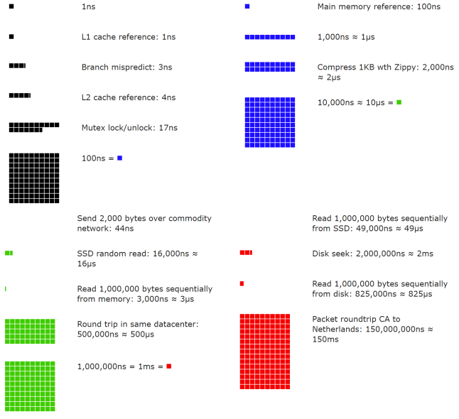
A Google software engineer built a tool to visualize Dr. Dean's numbers. The tool also takes the time factor into consideration. Figure 1 shows the visualized latency numbers as of 2020 (source of figures: reference material [3]).
Latency conclusions
By analyzing the numbers in Figure 1, we get the following conclusions:
- Memory is fast but the disk is slow. - Avoid disk seeks if possible. - Simple compression algorithms are fast. - Compress data before sending it over the internet if possible. - Data centers are usually in different regions, and it takes time to send data between them.
Availability numbers
High availability is the ability of a system to be continuously operational for a desirably long period of time. High availability is measured as a percentage, with 100% means a service that has 0 downtime. Most services fall between 99% and 100%.
A service level agreement (SLA) is a commonly used term for service providers. This is an agreement between you (the service provider) and your customer, and this agreement formally defines the level of uptime your service will deliver. Cloud providers Amazon [4], Google [5] and Microsoft [6] set their SLAs at 99.9% or above. Uptime is traditionally measured in nines. The more the nines, the better. As shown in Table 3, the number of nines correlate to the expected system downtime.
| Availability % | Downtime per day | Downtime per week | Downtime per month | Downtime per year | |----------------|------------------|-------------------|--------------------|-------------------| | 99% | 14.40 minutes | 1.68 hours | 7.31 hours | 3.65 days | | 99.9% | 1.44 minutes | 10.08 minutes | 43.83 minutes | 8.77 hours | | 99.99% | 8.64 seconds | 1.01 minutes | 4.38 minutes | 52.60 minutes | | 99.999% | 864.00 milliseconds | 6.05 seconds | 26.30 seconds | 5.26 minutes | | 99.9999% | 86.40 milliseconds | 604.80 milliseconds | 2.63 seconds | 31.56 seconds |
**Table 3: Availability numbers — the "nines"**
Example: Estimate Twitter QPS and storage requirements
Please note the following numbers are for this exercise only as they are not real numbers from Twitter.
**Assumptions:** - 300 million monthly active users. - 50% of users use Twitter daily. - Users post 2 tweets per day on average. - 10% of tweets contain media. - Data is stored for 5 years.
**Estimations:**
Query per second (QPS) estimate: - Daily active users (DAU) = 300 million × 50% = 150 million - Tweets QPS = 150 million × 2 tweets / 24 hour / 3600 seconds = ~3500 - Peak QPS = 2 × QPS = ~7000
We will only estimate media storage here.
Average tweet size: - tweet_id: 64 bytes - text: 140 bytes - media: 1 MB
Media storage: 150 million × 2 × 10% × 1 MB = **30 TB per day**
5-year media storage: 30 TB × 365 × 5 = **~55 PB**
Tips
Back-of-the-envelope estimation is all about the process. Solving the problem is more important than obtaining results. Interviewers may test your problem-solving skills. Here are a few tips to follow:
- **Rounding and Approximation.** It is difficult to perform complicated math operations during the interview. For example, what is the result of "99987 / 9.1"? There is no need to spend valuable time to solve complicated math problems. Precision is not expected. Use round numbers and approximation to your advantage. The division question can be simplified as follows: "100,000 / 10".
- **Write down your assumptions.** It is a good idea to write down your assumptions to be referenced later.
- **Label your units.** When you write down "5", does it mean 5 KB or 5 MB? You might confuse yourself with this. Write down the units because "5 MB" helps to remove ambiguity.
- **Commonly asked back-of-the-envelope estimations:** QPS, peak QPS, storage, cache, number of servers, etc. You can practice these calculations when preparing for an interview. Practice makes perfect.
A Framework For System Design Interviews
You have just landed a coveted on-site interview at your dream company. The hiring coordinator sends you a schedule for that day. Scanning down the list, you feel pretty good about it until your eyes land on this interview session — System Design Interview.
System design interviews are often intimidating. It could be as vague as "designing a well-known product X?". The questions are ambiguous and seem unreasonably broad. Your weariness is understandable. After all, how could anyone design a popular product in an hour that has taken hundreds if not thousands of engineers to build?
The good news is that no one expects you to. Real-world system design is extremely complicated. For example, Google search is deceptively simple; however, the amount of technology that underpins that simplicity is truly astonishing. If no one expects you to design a real-world system in an hour, what is the benefit of a system design interview?
The system design interview simulates real-life problem solving where two co-workers collaborate on an ambiguous problem and come up with a solution that meets their goals. The problem is open-ended, and there is no perfect answer. The final design is less important compared to the work you put in the design process. This allows you to demonstrate your design skill, defend your design choices, and respond to feedback in a constructive manner.
The primary goal of the interviewer is to accurately assess your abilities. An effective system design interview gives strong signals about a person's ability to collaborate, to work under pressure, and to resolve ambiguity constructively. The ability to ask good questions is also an essential skill, and many interviewers specifically look for this skill.
A good interviewer also looks for red flags. Over-engineering is a real disease of many engineers as they delight in design purity and ignore tradeoffs. They are often unaware of the compounding costs of over-engineered systems, and many companies pay a high price for that ignorance. Other red flags include narrow mindedness, stubbornness, etc.
In this chapter, we will go over some useful tips and introduce a simple and effective framework to solve system design interview problems.
A 4-step process for effective system design interview
Every system design interview is different. A great system design interview is open-ended and there is no one-size-fits-all solution. However, there are steps and common ground to cover in every system design interview.
Step 1 - Understand the problem and establish design scope
DON'T be like Jimmy — the student who always jumps to answer without fully understanding the question.
In a system design interview, giving out an answer quickly without thinking gives you no bonus points. Answering without a thorough understanding of the requirements is a huge red flag as the interview is not a trivia contest. There is no right answer.
So, do not jump right in to give a solution. Slow down. Think deeply and ask questions to clarify requirements and assumptions. This is extremely important.
As an engineer, we like to solve hard problems and jump into the final design; however, this approach is likely to lead you to design the wrong system. One of the most important skills as an engineer is to ask the right questions, make the proper assumptions, and gather all the information needed to build a system. So, do not be afraid to ask questions.
When you ask a question, the interviewer either answers your question directly or asks you to make your assumptions. If the latter happens, write down your assumptions on the whiteboard or paper. You might need them later.
**What kind of questions to ask?** Ask questions to understand the exact requirements. Here is a list of questions to help you get started:
- What specific features are we going to build? - How many users does the product have? - How fast does the company anticipate to scale up? What are the anticipated scales in 3 months, 6 months, and a year? - What is the company's technology stack? What existing services you might leverage to simplify the design?
**Example conversation for "Design a news feed system":**
> Candidate: Is this a mobile app? Or a web app? Or both? > Interviewer: Both. > > Candidate: What are the most important features for the product? > Interviewer: Ability to make a post and see friends' news feed. > > Candidate: Is the news feed sorted in reverse chronological order or a particular order? > Interviewer: To keep things simple, let us assume the feed is sorted by reverse chronological order. > > Candidate: How many friends can a user have? > Interviewer: 5000 > > Candidate: What is the traffic volume? > Interviewer: 10 million daily active users (DAU) > > Candidate: Can feed contain images, videos, or just text? > Interviewer: It can contain media files, including both images and videos.
Step 2 - Propose high-level design and get buy-in
In this step, we aim to develop a high-level design and reach an agreement with the interviewer on the design. It is a great idea to collaborate with the interviewer during the process.
- Come up with an initial blueprint for the design. Ask for feedback. Treat your interviewer as a teammate and work together. Many good interviewers love to talk and get involved. - Draw box diagrams with key components on the whiteboard or paper. This might include clients (mobile/web), APIs, web servers, data stores, cache, CDN, message queue, etc. - Do back-of-the-envelope calculations to evaluate if your blueprint fits the scale constraints. Think out loud. Communicate with your interviewer if back-of-the-envelope is necessary before diving into it. - If possible, go through a few concrete use cases. This will help you frame the high-level design. It is also likely that the use cases would help you discover edge cases you have not yet considered.
**Example — "Design a news feed system":**
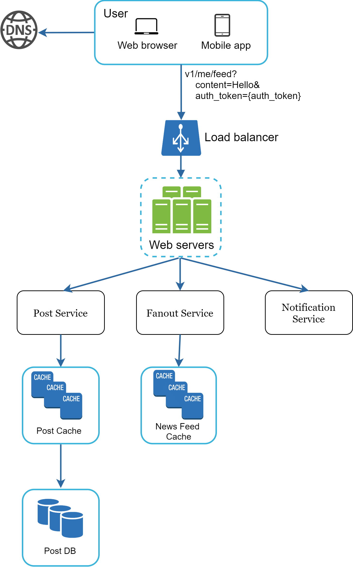
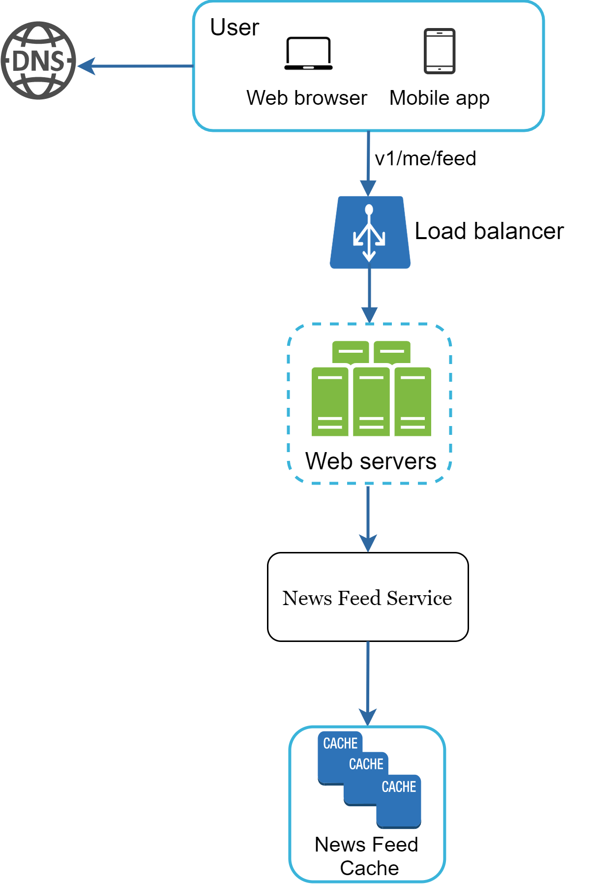
At the high level, the design is divided into two flows: feed publishing and news feed building.
- **Feed publishing:** when a user publishes a post, corresponding data is written into cache/database, and the post will be populated into friends' news feed. - **Newsfeed building:** the news feed is built by aggregating friends' posts in a reverse chronological order.
Figure 1 and Figure 2 present high-level designs for feed publishing and news feed building flows, respectively.
Step 3 - Design deep dive
At this step, you and your interviewer should have already achieved the following objectives:
- Agreed on the overall goals and feature scope - Sketched out a high-level blueprint for the overall design - Obtained feedback from your interviewer on the high-level design - Had some initial ideas about areas to focus on in deep dive based on her feedback
You shall work with the interviewer to identify and prioritize components in the architecture. It is worth stressing that every interview is different. Sometimes, the interviewer may give off hints that she likes focusing on high-level design. Sometimes, for a senior candidate interview, the discussion could be on the system performance characteristics, likely focusing on the bottlenecks and resource estimations. In most cases, the interviewer may want you to dig into details of some system components.
Time management is essential as it is easy to get carried away with minute details that do not demonstrate your abilities.
**Example — deep dive for news feed system:**
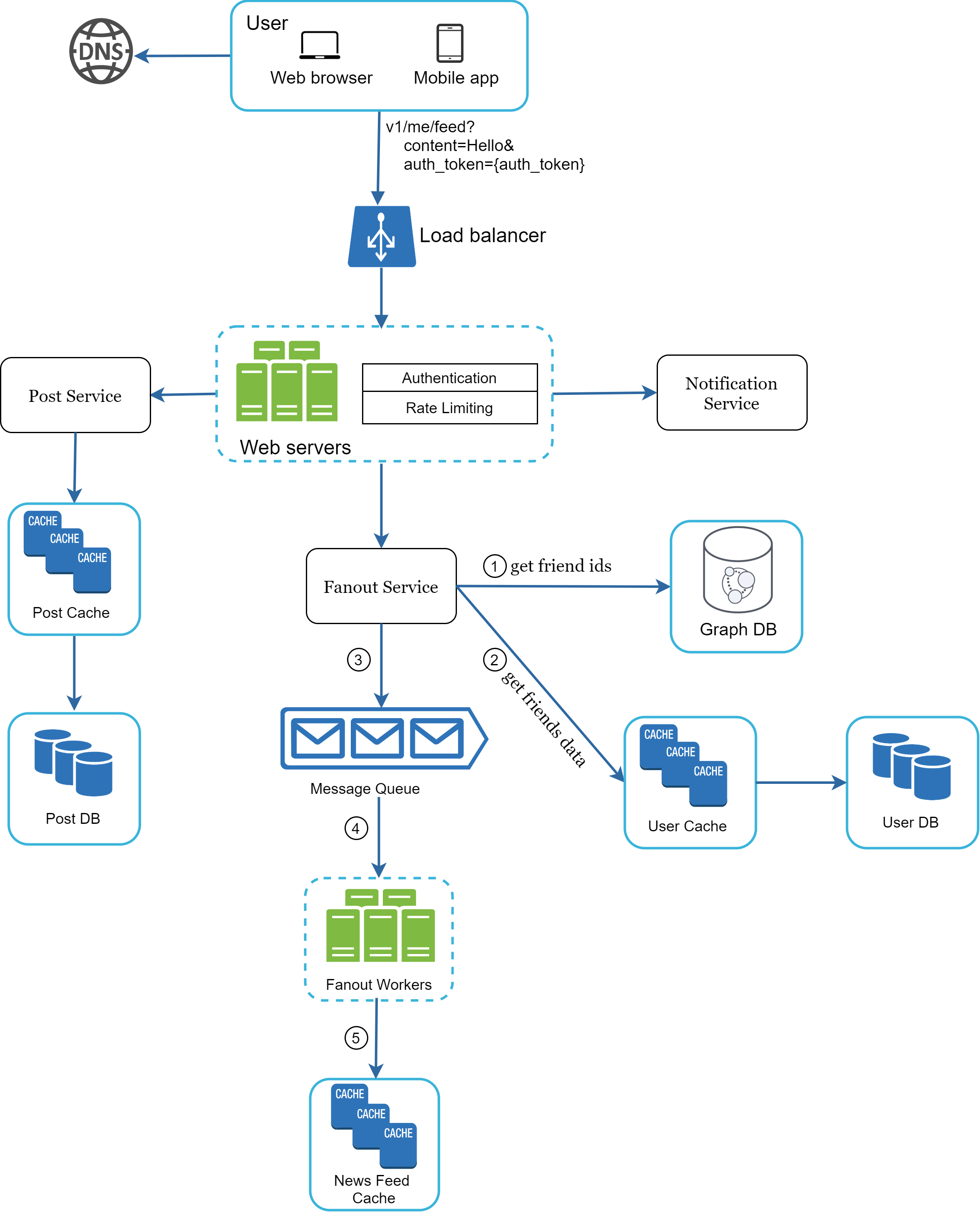
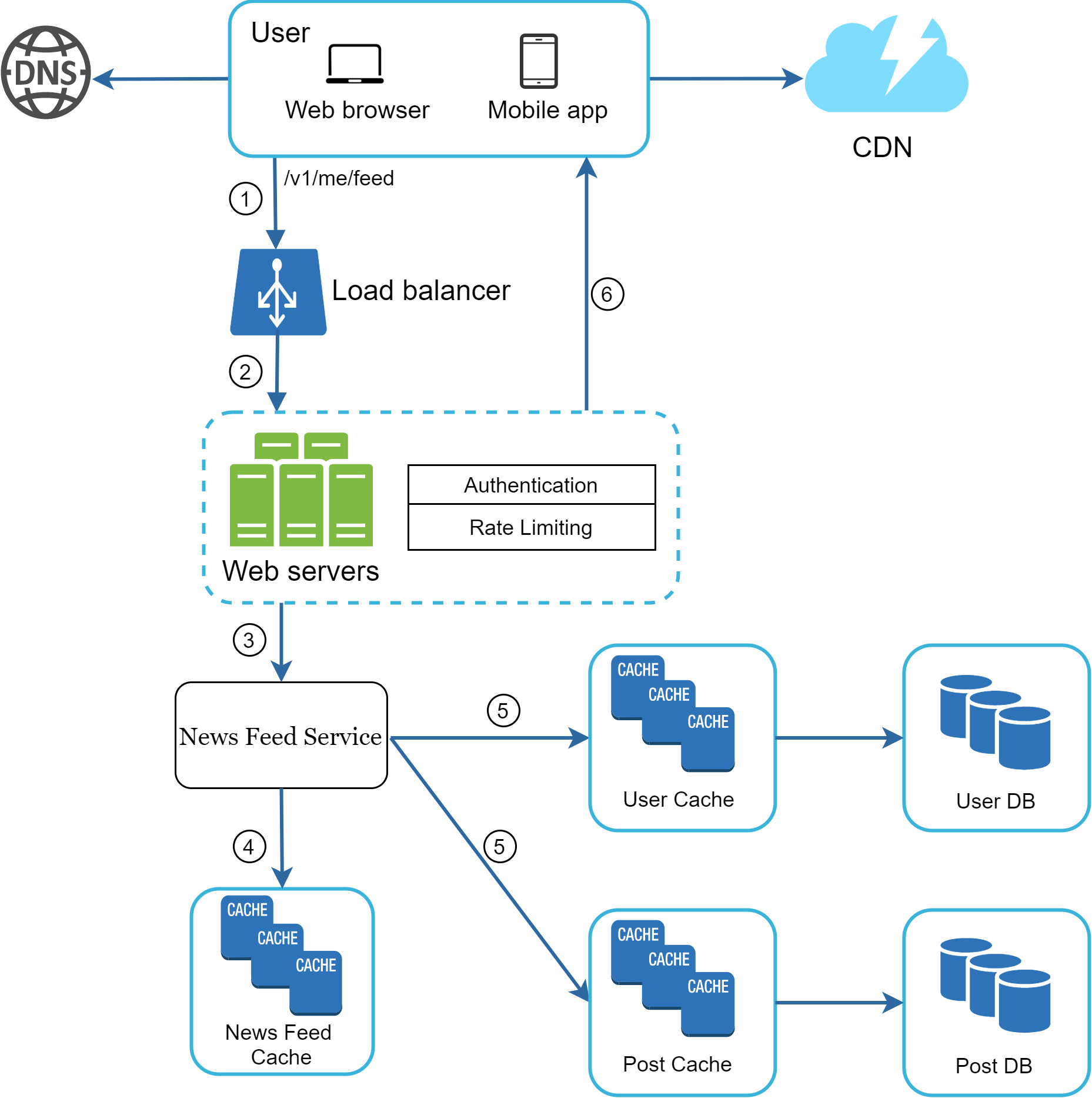
Figure 3 and Figure 4 show the detailed design for the feed publishing and news feed retrieval use cases, which will be explained in detail in the "Design A News Feed System" chapter.
Step 4 - Wrap up
In this final step, the interviewer might ask you a few follow-up questions or give you the freedom to discuss other additional points. Here are a few directions to follow:
- The interviewer might want you to identify the system bottlenecks and discuss potential improvements. Never say your design is perfect and nothing can be improved. There is always something to improve upon. - It could be useful to give the interviewer a recap of your design. This is particularly important if you suggested a few solutions. - Error cases (server failure, network loss, etc.) are interesting to talk about. - Operation issues are worth mentioning. How do you monitor metrics and error logs? How to roll out the system? - How to handle the next scale curve is also an interesting topic. For example, if your current design supports 1 million users, what changes do you need to make to support 10 million users? - Propose other refinements you need if you had more time.
Dos and Don'ts
**Dos:** - Always ask for clarification. Do not assume your assumption is correct. - Understand the requirements of the problem. - There is neither the right answer nor the best answer. A solution designed to solve the problems of a young startup is different from that of an established company with millions of users. - Let the interviewer know what you are thinking. Communicate with your interviewer. - Suggest multiple approaches if possible. - Once you agree with your interviewer on the blueprint, go into details on each component. Design the most critical components first. - Bounce ideas off the interviewer. A good interviewer works with you as a teammate. - Never give up.
**Don'ts:** - Don't be unprepared for typical interview questions. - Don't jump into a solution without clarifying the requirements and assumptions. - Don't go into too much detail on a single component in the beginning. Give the high-level design first then drills down. - If you get stuck, don't hesitate to ask for hints. - Again, communicate. Don't think in silence. - Don't think your interview is done once you give the design. You are not done until your interviewer says you are done. Ask for feedback early and often.
Time allocation on each step
System design interview questions are usually very broad, and 45 minutes or an hour is not enough to cover the entire design. Time management is essential. The following is a very rough guide on distributing your time in a 45-minute interview session:
- **Step 1** — Understand the problem and establish design scope: **3–10 minutes** - **Step 2** — Propose high-level design and get buy-in: **10–15 minutes** - **Step 3** — Design deep dive: **10–25 minutes** - **Step 4** — Wrap up: **3–5 minutes**
Design A Rate Limiter
In a network system, a rate limiter is used to control the rate of traffic sent by a client or a service. In the HTTP world, a rate limiter limits the number of client requests allowed to be sent over a specified period. If the API request count exceeds the threshold defined by the rate limiter, all the excess calls are blocked. Here are a few examples:
- A user can write no more than 2 posts per second. - You can create a maximum of 10 accounts per day from the same IP address. - You can claim rewards no more than 5 times per week from the same device.
**Benefits of using an API rate limiter:**
- **Prevent resource starvation caused by DoS attack [1].** Almost all APIs published by large tech companies enforce some form of rate limiting. For example, Twitter limits the number of tweets to 300 per 3 hours [2]. Google docs APIs have the following default limit: 300 per user per 60 seconds for read requests [3]. A rate limiter prevents DoS attacks, either intentional or unintentional, by blocking the excess calls. - **Reduce cost.** Limiting excess requests means fewer servers and allocating more resources to high priority APIs. Rate limiting is extremely important for companies that use paid third party APIs. - **Prevent servers from being overloaded.** To reduce server load, a rate limiter is used to filter out excess requests caused by bots or users' misbehavior.
Step 1 - Understand the problem and establish design scope
Rate limiting can be implemented using different algorithms, each with its pros and cons.
**Requirements summary:**
- Accurately limit excessive requests. - Low latency. The rate limiter should not slow down HTTP response time. - Use as little memory as possible. - Distributed rate limiting. The rate limiter can be shared across multiple servers or processes. - Exception handling. Show clear exceptions to users when their requests are throttled. - High fault tolerance. If there are any problems with the rate limiter (for example, a cache server goes offline), it does not affect the entire system.
Step 2 - Propose high-level design and get buy-in
Let us keep things simple and use a basic client and server model for communication.
Where to put the rate limiter?
Intuitively, you can implement a rate limiter at either the client or server-side.
- **Client-side implementation.** Generally speaking, client is an unreliable place to enforce rate limiting because client requests can easily be forged by malicious actors. Moreover, we might not have control over the client implementation.
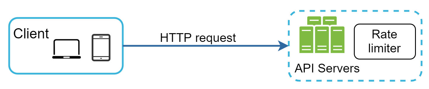
- **Server-side implementation.** Figure 1 shows a rate limiter that is placed on the server-side.
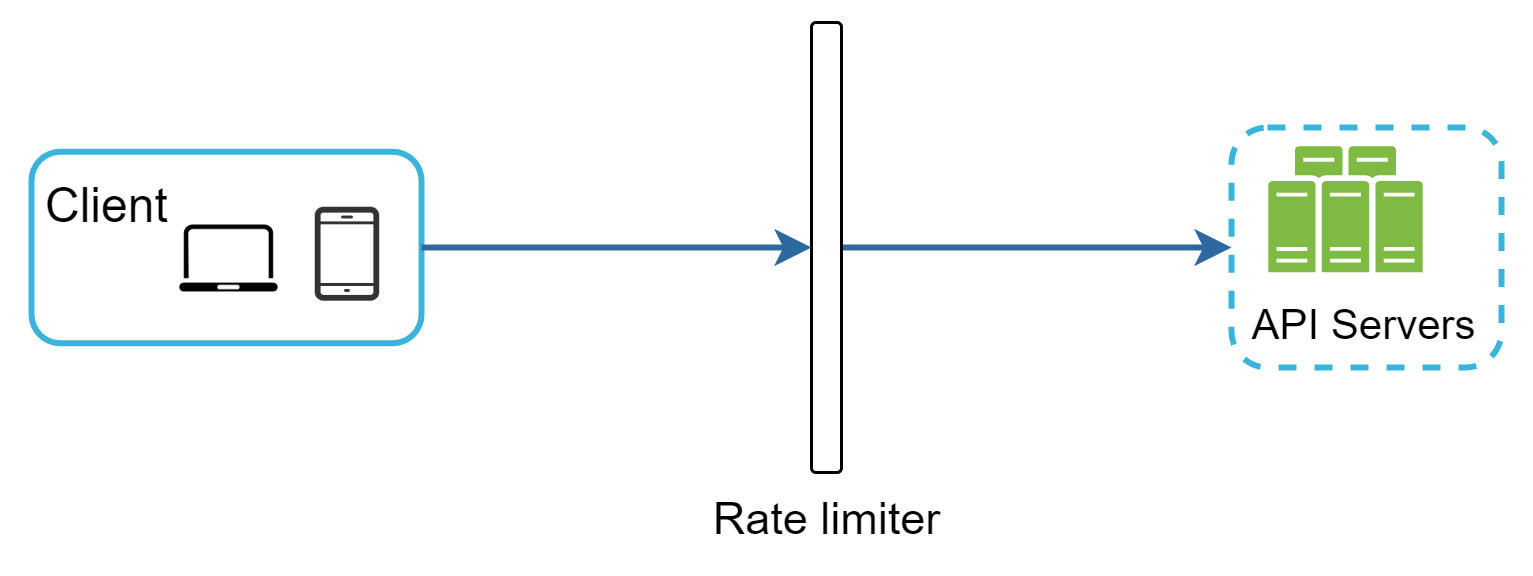
Besides the client and server-side implementations, there is an alternative way. Instead of putting a rate limiter at the API servers, we create a rate limiter middleware, which throttles requests to your APIs as shown in Figure 2.
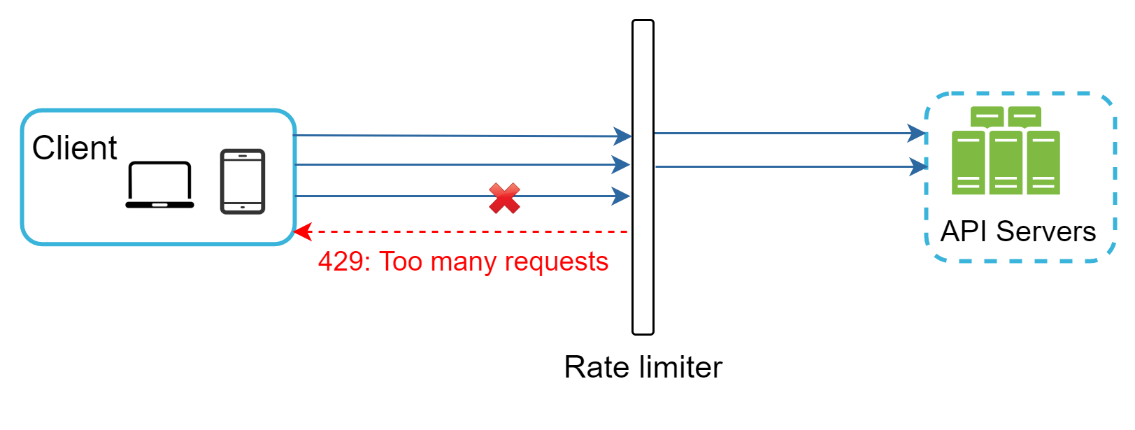
Figure 3 illustrates how rate limiting works: assume our API allows 2 requests per second, and a client sends 3 requests to the server within a second. The first two requests are routed to API servers. However, the rate limiter middleware throttles the third request and returns a HTTP status code 429.
Cloud microservices [4] have become widely popular and rate limiting is usually implemented within a component called API gateway. API gateway is a fully managed service that supports rate limiting, SSL termination, authentication, IP whitelisting, servicing static content, etc.
**General guidelines for placement:**
- Evaluate your current technology stack, such as programming language, cache service, etc. - Identify the rate limiting algorithm that fits your business needs. - If you have already used microservice architecture and included an API gateway, you may add a rate limiter to the API gateway. - Building your own rate limiting service takes time. If you do not have enough engineering resources, a commercial API gateway is a better option.
Algorithms for rate limiting
Rate limiting can be implemented using different algorithms, and each of them has distinct pros and cons. Here is a list of popular algorithms:
- Token bucket - Leaking bucket - Fixed window counter - Sliding window log - Sliding window counter
Token bucket algorithm
The token bucket algorithm is widely used for rate limiting. It is simple, well understood and commonly used by internet companies. Both Amazon [5] and Stripe [6] use this algorithm to throttle their API requests.
**How it works:** - A token bucket is a container that has pre-defined capacity. Tokens are put in the bucket at preset rates periodically. Once the bucket is full, no more tokens are added. As shown in Figure 4, the token bucket capacity is 4. The refiller puts 2 tokens into the bucket every second. Once the bucket is full, extra tokens will overflow. - Each request consumes one token. When a request arrives, we check if there are enough tokens in the bucket (Figure 5). - If there are enough tokens, we take one token out for each request, and the request goes through. - If there are not enough tokens, the request is dropped. - Figure 6 illustrates how token consumption, refill, and rate limiting logic work. In this example, the token bucket size is 4, and the refill rate is 4 per 1 minute.
**Parameters:** - **Bucket size:** the maximum number of tokens allowed in the bucket - **Refill rate:** number of tokens put into the bucket every second
**Pros:** - The algorithm is easy to implement. - Memory efficient. - Token bucket allows a burst of traffic for short periods. A request can go through as long as there are tokens left.
**Cons:** - Two parameters in the algorithm are bucket size and token refill rate. However, it might be challenging to tune them properly.


Leaking bucket algorithm
The leaking bucket algorithm is similar to the token bucket except that requests are processed at a fixed rate. It is usually implemented with a first-in-first-out (FIFO) queue.
**How it works:** - When a request arrives, the system checks if the queue is full. If it is not full, the request is added to the queue. - Otherwise, the request is dropped. - Requests are pulled from the queue and processed at regular intervals.
Figure 7 explains how the algorithm works.
**Parameters:** - **Bucket size:** equal to the queue size. The queue holds the requests to be processed at a fixed rate. - **Outflow rate:** defines how many requests can be processed at a fixed rate, usually in seconds.
Shopify, an ecommerce company, uses leaky buckets for rate-limiting [7].
**Pros:** - Memory efficient given the limited queue size. - Requests are processed at a fixed rate therefore it is suitable for use cases that a stable outflow rate is needed.
**Cons:** - A burst of traffic fills up the queue with old requests, and if they are not processed in time, recent requests will be rate limited. - There are two parameters in the algorithm. It might not be easy to tune them properly.

Fixed window counter algorithm
**How it works:** - The algorithm divides the timeline into fix-sized time windows and assign a counter for each window. - Each request increments the counter by one. - Once the counter reaches the pre-defined threshold, new requests are dropped until a new time window starts.
In Figure 8, the time unit is 1 second and the system allows a maximum of 3 requests per second.
A major problem with this algorithm is that a burst of traffic at the edges of time windows could cause more requests than allowed quota to go through. As seen in Figure 9, there are five requests between 2:00:00 and 2:01:00 and five more requests between 2:01:00 and 2:02:00. For the one-minute window between 2:00:30 and 2:01:30, 10 requests go through — twice as many as allowed.
**Pros:** - Memory efficient. - Easy to understand. - Resetting available quota at the end of a unit time window fits certain use cases.
**Cons:** - Spike in traffic at the edges of a window could cause more requests than the allowed quota to go through.


Sliding window log algorithm
The sliding window log algorithm fixes the edge-burst issue of fixed window counter.
**How it works:** 1. The algorithm keeps track of request timestamps. Timestamp data is usually kept in cache, such as sorted sets of Redis [8]. 2. When a new request comes in, remove all the outdated timestamps. Outdated timestamps are defined as those older than the start of the current time window. 3. Add timestamp of the new request to the log. 4. If the log size is the same or lower than the allowed count, a request is accepted. Otherwise, it is rejected.
Figure 10 explains the algorithm with an example (rate limit: 2 requests per minute): - **1:00:01** — Log is empty, request is allowed. - **1:00:30** — Timestamp inserted, log size = 2, request is allowed. - **1:00:50** — Timestamp inserted, log size = 3 > 2, request is rejected. - **1:01:40** — Outdated timestamps 1:00:01 and 1:00:30 removed. Log size = 2, request is accepted.
**Pros:** - Rate limiting is very accurate. In any rolling window, requests will not exceed the rate limit.
**Cons:** - The algorithm consumes a lot of memory because even if a request is rejected, its timestamp might still be stored in memory.

Sliding window counter algorithm
The sliding window counter algorithm is a hybrid approach that combines the fixed window counter and sliding window log.
Figure 11 illustrates how this algorithm works. Assume the rate limiter allows a maximum of 7 requests per minute, and there are 5 requests in the previous minute and 3 in the current minute. For a new request that arrives at a 30% position in the current minute:
``` Requests in current window + requests in the previous window × overlap percentage = 3 + 5 × 0.7 = 6.5 → rounded down to 6 ```
Since the rate limiter allows a maximum of 7 requests per minute, the current request can go through.
**Pros:** - It smooths out spikes in traffic because the rate is based on the average rate of the previous window. - Memory efficient.
**Cons:** - It only works for not-so-strict look back window. It is an approximation of the actual rate. However, according to experiments done by Cloudflare [10], only 0.003% of requests are wrongly allowed or rate limited among 400 million requests.

High-level architecture
The basic idea of rate limiting algorithms is simple. At the high-level, we need a counter to keep track of how many requests are sent from the same user, IP address, etc. If the counter is larger than the limit, the request is disallowed.
**Where shall we store counters?** Using the database is not a good idea due to slowness of disk access. In-memory cache is chosen because it is fast and supports time-based expiration strategy. Redis [11] is a popular option to implement rate limiting. It is an in-memory store that offers two commands:
- **INCR:** Increases the stored counter by 1. - **EXPIRE:** Sets a timeout for the counter. If the timeout expires, the counter is automatically deleted.
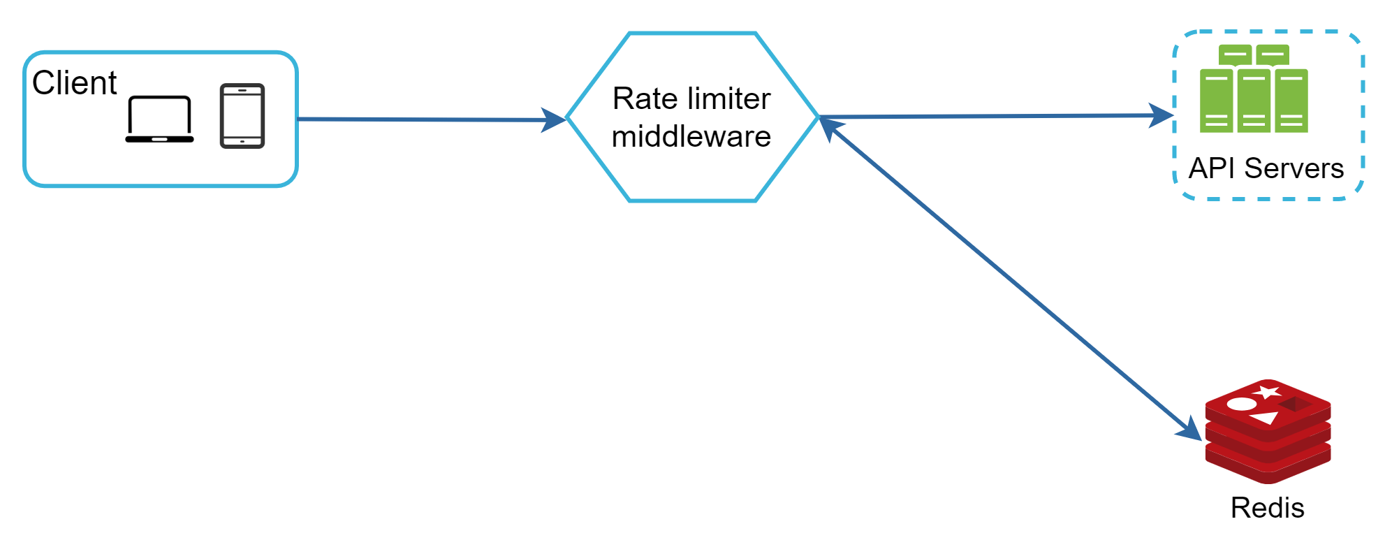
Figure 12 shows the high-level architecture for rate limiting: 1. The client sends a request to rate limiting middleware. 2. Rate limiting middleware fetches the counter from the corresponding bucket in Redis and checks if the limit is reached or not. 3. If the limit is reached, the request is rejected. 4. If the limit is not reached, the request is sent to API servers. Meanwhile, the system increments the counter and saves it back to Redis.
Step 3 - Design deep dive
Rate limiting rules
Lyft open-sourced their rate-limiting component [12]. Example rate limiting rules:
```yaml domain: messaging descriptors: - key: message_type value: marketing rate_limit: unit: day requests_per_unit: 5 ```
This allows a maximum of 5 marketing messages per day.
```yaml domain: auth descriptors: - key: auth_type value: login rate_limit: unit: minute requests_per_unit: 5 ```
This rule limits login to no more than 5 times per minute. Rules are generally written in configuration files and saved on disk.
Exceeding the rate limit
In case a request is rate limited, APIs return a HTTP response code **429 (too many requests)** to the client. Depending on the use cases, we may enqueue the rate-limited requests to be processed later.
**Rate limiter headers** — how clients know they are being throttled:
- `X-Ratelimit-Remaining` — The remaining number of allowed requests within the window. - `X-Ratelimit-Limit` — How many calls the client can make per time window. - `X-Ratelimit-Retry-After` — The number of seconds to wait until you can make a request again without being throttled.
Detailed design
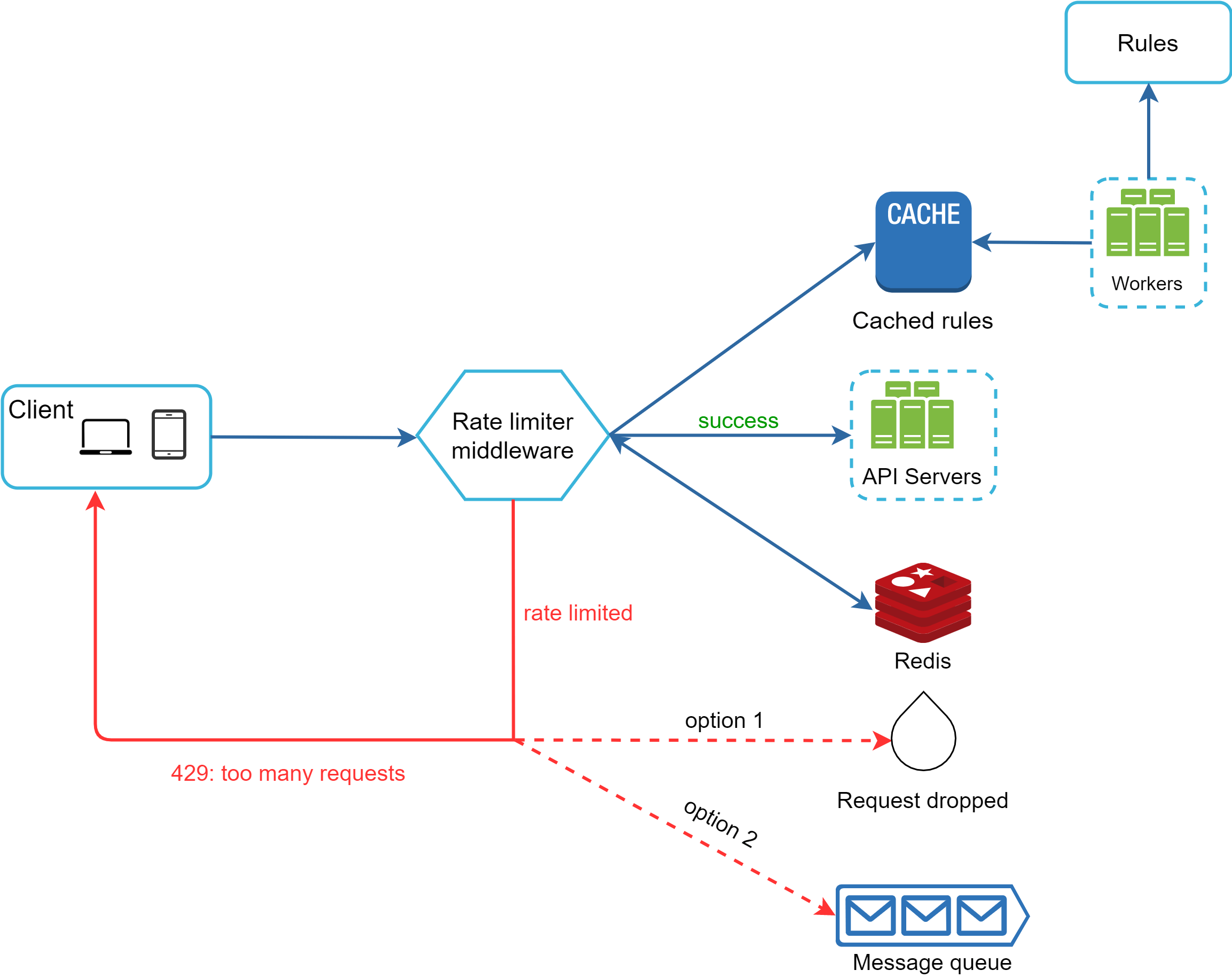
Figure 13 presents a detailed design of the system.
- Rules are stored on the disk. Workers frequently pull rules from the disk and store them in the cache. - When a client sends a request to the server, the request is sent to the rate limiter middleware first. - Rate limiter middleware loads rules from the cache. It fetches counters and last request timestamp from Redis cache. Based on the response, the rate limiter decides: - if the request is not rate limited, it is forwarded to API servers. - if the request is rate limited, the rate limiter returns 429 too many requests error to the client. In the meantime, the request is either dropped or forwarded to the queue.
Rate limiter in a distributed environment
Building a rate limiter that works in a single server environment is not difficult. However, scaling the system to support multiple servers and concurrent threads is a different story. There are two challenges:
**1. Race condition**
Rate limiter works as follows at the high-level: read the counter value from Redis, check if (counter + 1) exceeds the threshold, if not, increment the counter value by 1 in Redis.
Race conditions can happen in a highly concurrent environment as shown in Figure 14. If two requests concurrently read the counter value (3) before either of them writes back, each will increment to 4 instead of the correct value 5.
Locks are the most obvious solution for solving race condition. However, locks will significantly slow down the system. Two strategies are commonly used: Lua script [13] and sorted sets data structure in Redis [8].
**2. Synchronization issue**
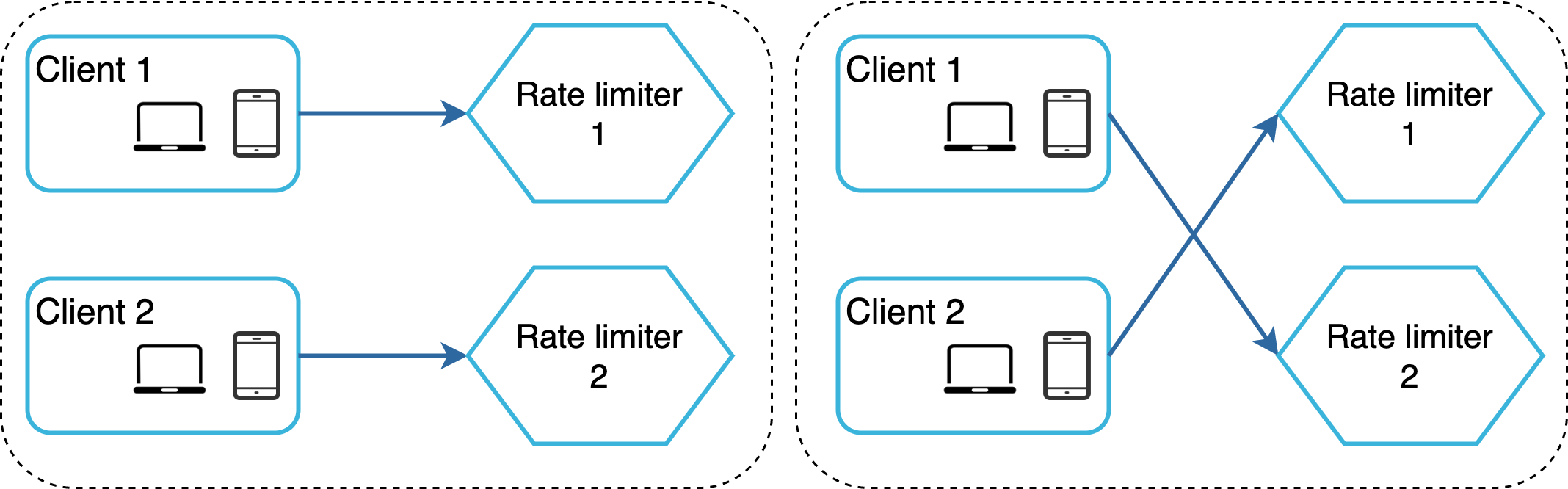
To support millions of users, one rate limiter server might not be enough to handle the traffic. When multiple rate limiter servers are used, synchronization is required.
As shown in Figure 15, if client 1 sends requests to rate limiter 1 and client 2 sends requests to rate limiter 2, rate limiter 1 does not contain any data about client 2.
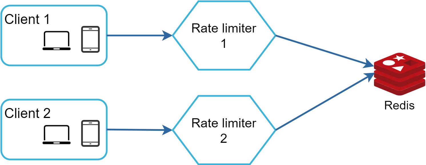
One possible solution is to use sticky sessions. However, a better approach is to use centralized data stores like Redis, as shown in Figure 16.

Performance optimization
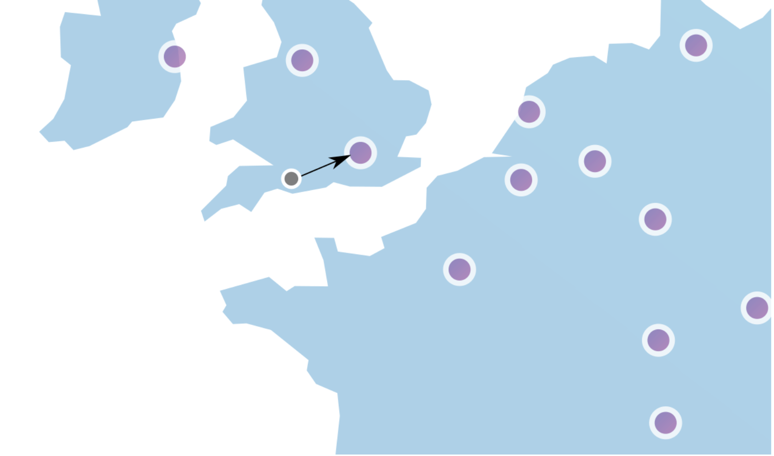
**First:** Multi-data center setup is crucial for a rate limiter because latency is high for users located far away from the data center. Most cloud service providers build many edge server locations around the world. Traffic is automatically routed to the closest edge server to reduce latency.
**Second:** Synchronize data with an eventual consistency model.
Monitoring
After the rate limiter is put in place, it is important to gather analytics data to check whether the rate limiter is effective. Primarily, we want to make sure:
- The rate limiting algorithm is effective. - The rate limiting rules are effective.
For example, if rate limiting rules are too strict, many valid requests are dropped. In this case, we want to relax the rules a little bit. In another example, if the rate limiter becomes ineffective when there is a sudden increase in traffic like flash sales, we may replace the algorithm to support burst traffic. Token bucket is a good fit here.
Step 4 - Wrap up
In this chapter, we discussed different algorithms of rate limiting and their pros/cons:
- **Token bucket** — allows bursts, easy to implement - **Leaking bucket** — stable outflow, good for streaming - **Fixed window** — simple, but edge-burst problem - **Sliding window log** — accurate, memory-intensive - **Sliding window counter** — approximate but memory efficient
**Additional talking points:**
- **Hard vs soft rate limiting:** - Hard: The number of requests cannot exceed the threshold. - Soft: Requests can exceed the threshold for a short period.
- **Rate limiting at different levels.** In this chapter, we only talked about rate limiting at the application level (HTTP: layer 7). It is possible to apply rate limiting at other layers. For example, you can apply rate limiting by IP addresses using Iptables [15] (IP: layer 3).
- **Avoid being rate limited — client best practices:** - Use client cache to avoid making frequent API calls. - Understand the limit and do not send too many requests in a short time frame. - Include code to catch exceptions or errors so your client can gracefully recover from exceptions. - Add sufficient back off time to retry logic.
Design Consistent Hashing
To achieve horizontal scaling, it is important to distribute requests/data efficiently and evenly across servers. Consistent hashing is a commonly used technique to achieve this goal.
The rehashing problem
If you have n cache servers, a common way to balance the load is to use the following hash method:
``` serverIndex = hash(key) % N, where N is the size of the server pool. ```
With 4 servers and 8 string keys (Table 1), to fetch the server where a key is stored, we perform the modular operation `f(key) % 4`. Figure 1 shows the distribution of keys based on Table 1.
| key | hash | hash % 4 | |-----|------|----------| | key0 | 18358617 | 1 | | key1 | 26143584 | 0 | | key2 | 18131146 | 2 | | key3 | 35863496 | 0 | | key4 | 34085809 | 1 | | key5 | 27581703 | 3 | | key6 | 38164978 | 2 | | key7 | 22530351 | 3 |
**Table 1**
This approach works well when the size of the server pool is fixed, and the data distribution is even. However, problems arise when new servers are added, or existing servers are removed. For example, if server 1 goes offline, the size of the server pool becomes 3. Applying modular operation gives us different server indexes because the number of servers is reduced by 1.
| key | hash | hash % 3 | |-----|------|----------| | key0 | 18358617 | 0 | | key1 | 26143584 | 0 | | key2 | 18131146 | 1 | | key3 | 35863496 | 2 | | key4 | 34085809 | 1 | | key5 | 27581703 | 0 | | key6 | 38164978 | 1 | | key7 | 22530351 | 0 |
**Table 2**
As shown in Figure 2, most keys are redistributed, not just the ones originally stored in the offline server. This means that when server 1 goes offline, most cache clients will connect to the wrong servers to fetch data. This causes a storm of cache misses. Consistent hashing is an effective technique to mitigate this problem.


Consistent hashing
Quoted from Wikipedia: "Consistent hashing is a special kind of hashing such that when a hash table is re-sized and consistent hashing is used, only k/n keys need to be remapped on average, where k is the number of keys, and n is the number of slots. In contrast, in most traditional hash tables, a change in the number of array slots causes nearly all keys to be remapped [1]".
Hash space and hash ring
Assume SHA-1 is used as the hash function f, and the output range of the hash function is: x0, x1, x2, x3, …, xn. In cryptography, SHA-1's hash space goes from 0 to 2^160 - 1. That means x0 corresponds to 0, xn corresponds to 2^160 – 1. Figure 3 shows the hash space.
By collecting both ends, we get a hash ring as shown in Figure 4.


Hash servers
Using the same hash function f, we map servers based on server IP or name onto the ring. Figure 5 shows that 4 servers are mapped on the hash ring.

Hash keys
The hash function used here is different from the one in "the rehashing problem," and there is no modular operation. As shown in Figure 6, 4 cache keys (key0, key1, key2, and key3) are hashed onto the hash ring.

Server lookup
To determine which server a key is stored on, we go clockwise from the key position on the ring until a server is found. Figure 7 explains this process: going clockwise, key0 is stored on server 0; key1 is stored on server 1; key2 is stored on server 2 and key3 is stored on server 3.

Add a server
Using the logic described above, adding a new server will only require redistribution of a fraction of keys.
In Figure 8, after a new server 4 is added, only key0 needs to be redistributed. k1, k2, and k3 remain on the same servers. Before server 4 is added, key0 is stored on server 0. Now, key0 will be stored on server 4 because server 4 is the first server it encounters by going clockwise from key0's position on the ring.

Remove a server
When a server is removed, only a small fraction of keys require redistribution with consistent hashing. In Figure 9, when server 1 is removed, only key1 must be remapped to server 2. The rest of the keys are unaffected.

Two issues in the basic approach
The consistent hashing algorithm was introduced by Karger et al. at MIT [1]. The basic steps are:
1. Map servers and keys on to the ring using a uniformly distributed hash function. 2. To find out which server a key is mapped to, go clockwise from the key position until the first server on the ring is found.
**Problem 1: Non-uniform partitions.** It is impossible to keep the same size of partitions on the ring for all servers considering a server can be added or removed. In Figure 10, if s1 is removed, s2's partition is twice as large as s0 and s3's partition.
**Problem 2: Non-uniform key distribution.** If servers are mapped to positions listed in Figure 11, most of the keys are stored on server 2. However, server 1 and server 3 have no data.
A technique called **virtual nodes** or replicas is used to solve these problems.


Virtual nodes
A virtual node refers to the real node, and each server is represented by multiple virtual nodes on the ring. In Figure 12, both server 0 and server 1 have 3 virtual nodes. Instead of using s0, we have s0_0, s0_1, and s0_2 to represent server 0 on the ring. Similarly, s1_0, s1_1, and s1_2 represent server 1 on the ring. With virtual nodes, each server is responsible for multiple partitions.
To find which server a key is stored on, we go clockwise from the key's location and find the first virtual node encountered on the ring. In Figure 13, to find out which server k0 is stored on, we go clockwise from k0's location and find virtual node s1_1, which refers to server 1.
As the number of virtual nodes increases, the distribution of keys becomes more balanced because the standard deviation gets smaller. According to online research [2], with one or two hundred virtual nodes, the standard deviation is between 5% (200 virtual nodes) and 10% (100 virtual nodes) of the mean. However, more spaces are needed to store data about virtual nodes. This is a tradeoff.


Find affected keys
When a server is added or removed, a fraction of data needs to be redistributed.
In Figure 14, server 4 is added onto the ring. The affected range starts from s4 (newly added node) and moves anticlockwise around the ring until a server is found (s3). Thus, keys located between s3 and s4 need to be redistributed to s4.
When a server (s1) is removed as shown in Figure 15, the affected range starts from s1 (removed node) and moves anticlockwise around the ring until a server is found (s0). Thus, keys located between s0 and s1 must be redistributed to s2.


Wrap up
The benefits of consistent hashing include:
- **Minimized redistribution** when servers are added or removed. - **Easy to scale horizontally** because data are more evenly distributed. - **Mitigate hotspot key problem.** Excessive access to a specific shard could cause server overload. Consistent hashing helps to mitigate the problem by distributing the data more evenly.
Consistent hashing is widely used in real-world systems:
- Partitioning component of Amazon's Dynamo database [3] - Data partitioning across the cluster in Apache Cassandra [4] - Discord chat application [5] - Akamai content delivery network [6] - Maglev network load balancer [7]
Design A Key-value Store
A key-value store, also referred to as a key-value database, is a non-relational database. Each unique identifier is stored as a key with its associated value. This data pairing is known as a "key-value" pair.
In a key-value pair, the key must be unique, and the value associated with the key can be accessed through the key. Keys can be plain text or hashed values. For performance reasons, a short key works better.
- Plain text key: `"last_logged_in_at"` - Hashed key: `253DDEC4`
The value in a key-value pair can be strings, lists, objects, etc. The value is usually treated as an opaque object in key-value stores, such as Amazon DynamoDB [1], Memcached [2], Redis [3], etc.
In this chapter, you are asked to design a key-value store that supports the following operations:
- `put(key, value)` — insert "value" associated with "key" - `get(key)` — get "value" associated with "key"
Understand the problem and establish design scope
There is no perfect design. Each design achieves a specific balance regarding the tradeoffs of the read, write, and memory usage. Another tradeoff has to be made between consistency and availability. In this chapter, we design a key-value store that comprises of the following characteristics:
- The size of a key-value pair is small: less than 10 KB. - Ability to store big data. - High availability: The system responds quickly, even during failures. - High scalability: The system can be scaled to support large data set. - Automatic scaling: The addition/deletion of servers should be automatic based on traffic. - Tunable consistency. - Low latency.
Single server key-value store
Developing a key-value store that resides in a single server is easy. An intuitive approach is to store key-value pairs in a hash table, which keeps everything in memory. Even though memory access is fast, fitting everything in memory may be impossible due to the space constraint. Two optimizations can be done to fit more data in a single server:
- Data compression - Store only frequently used data in memory and the rest on disk
Even with these optimizations, a single server can reach its capacity very quickly. A distributed key-value store is required to support big data.
Distributed key-value store
A distributed key-value store is also called a distributed hash table, which distributes key-value pairs across many servers. When designing a distributed system, it is important to understand CAP (Consistency, Availability, Partition Tolerance) theorem.
CAP theorem
CAP theorem states it is impossible for a distributed system to simultaneously provide more than two of these three guarantees: consistency, availability, and partition tolerance.
- **Consistency:** all clients see the same data at the same time no matter which node they connect to. - **Availability:** any client which requests data gets a response even if some of the nodes are down. - **Partition Tolerance:** the system continues to operate despite network partitions (communication breaks between nodes).
CAP theorem states that one of the three properties must be sacrificed to support 2 of the 3 properties as shown in Figure 1.
Key-value stores are classified based on the two CAP characteristics they support:
- **CP systems:** support consistency and partition tolerance while sacrificing availability. - **AP systems:** support availability and partition tolerance while sacrificing consistency. - **CA systems:** support consistency and availability while sacrificing partition tolerance. Since network failure is unavoidable, a distributed system must tolerate network partition. Thus, a CA system cannot exist in real-world applications.
**Ideal situation (Figure 2):** Network partition never occurs. Data written to n1 is automatically replicated to n2 and n3. Both consistency and availability are achieved.
**Real-world (Figure 3):** n3 goes down and cannot communicate with n1 and n2. We must choose between: - **CP system:** block all write operations to n1 and n2 to avoid data inconsistency, making the system temporarily unavailable. Bank systems typically require this. - **AP system:** keep accepting reads (potentially stale) and writes, sync data to n3 when the partition resolves.


System components
Core components and techniques used to build a key-value store:
- Data partition - Data replication - Consistency - Inconsistency resolution - Handling failures - System architecture diagram - Write path - Read path
The content below is largely based on three popular key-value store systems: Dynamo [4], Cassandra [5], and BigTable [6].
Data partition
For large applications, it is infeasible to fit the complete data set in a single server. Consistent hashing is a great technique to partition data:
1. Servers are placed on a hash ring. In Figure 4, eight servers (s0–s7) are placed on the hash ring. 2. A key is hashed onto the same ring, and it is stored on the first server encountered while moving clockwise. For instance, key0 is stored in s1.
Advantages: - **Automatic scaling:** servers could be added and removed automatically depending on the load. - **Heterogeneity:** the number of virtual nodes for a server is proportional to the server capacity.

Data replication
To achieve high availability and reliability, data must be replicated asynchronously over N servers (N is a configurable parameter). After a key is mapped to a position on the hash ring, walk clockwise from that position and choose the first N servers on the ring to store data copies. In Figure 5 (N = 3), key0 is replicated at s1, s2, and s3.
With virtual nodes, the first N nodes on the ring may be owned by fewer than N physical servers. To avoid this issue, we only choose unique servers while performing the clockwise walk logic.
For better reliability, replicas are placed in distinct data centers, and data centers are connected through high-speed networks.

Consistency
Since data is replicated at multiple nodes, it must be synchronized across replicas. Quorum consensus can guarantee consistency for both read and write operations.
**Definitions:** - **N** = The number of replicas - **W** = A write quorum of size W. For a write operation to be considered as successful, write operation must be acknowledged from W replicas. - **R** = A read quorum of size R. For a read operation to be considered as successful, read operation must wait for responses from at least R replicas.
Figure 6 shows an example with N = 3. W = 1 means that the coordinator must receive at least one acknowledgment before the write operation is considered successful. A coordinator acts as a proxy between the client and the nodes.
**Configuration tradeoffs:** - If R = 1 and W = N: optimized for fast read. - If W = 1 and R = N: optimized for fast write. - If W + R > N: strong consistency guaranteed (Usually N = 3, W = R = 2). - If W + R ≤ N: strong consistency is not guaranteed.

Consistency models
A consistency model defines the degree of data consistency:
- **Strong consistency:** any read operation returns a value corresponding to the result of the most updated write data item. A client never sees out-of-date data. - **Weak consistency:** subsequent read operations may not see the most updated value. - **Eventual consistency:** a specific form of weak consistency. Given enough time, all updates are propagated, and all replicas are consistent.
Strong consistency is usually achieved by forcing a replica not to accept new reads/writes until every replica has agreed on current write — not ideal for highly available systems. Dynamo and Cassandra adopt **eventual consistency**, which is our recommended consistency model.
Inconsistency resolution: versioning
Replication gives high availability but causes inconsistencies among replicas. Versioning and vector locks are used to solve inconsistency problems.
As shown in Figure 7, both replica nodes n1 and n2 have the same value (original value). Server 1 changes the name to "johnSanFrancisco", and server 2 changes the name to "johnNewYork" simultaneously as shown in Figure 8. This creates conflicting versions v1 and v2.
**Vector clock** is a common technique to resolve this problem. A vector clock is a [server, version] pair associated with a data item. It can be used to check if one version precedes, succeeds, or is in conflict with others.
Assume a vector clock is represented by D([S1, v1], [S2, v2], …, [Sn, vn]). If data item D is written to server Si: - Increment vi if [Si, vi] exists. - Otherwise, create a new entry [Si, 1].
Figure 9 illustrates the vector clock process: 1. Client writes D1 to server Sx → vector clock D1[(Sx, 1)] 2. Another client reads D1, updates to D2, writes back to Sx → D2([Sx, 2]) 3. Another client reads D2, updates to D3, writes to Sy → D3([Sx, 2], [Sy, 1]) 4. Another client reads D2, updates to D4, writes to Sz → D4([Sx, 2], [Sz, 1]) 5. A client reads D3 and D4, discovers a conflict (D2 was modified by both Sy and Sz). Client resolves conflict and sends D5 → D5([Sx, 3], [Sy, 1], [Sz, 1])
**Version X is an ancestor of Y** (no conflict) if all version counters in X are ≤ corresponding counters in Y. **Version X is a sibling of Y** (conflict) if there is any participant in Y's vector clock with a counter less than its corresponding counter in X.
**Downsides of vector clocks:** 1. Adds complexity to the client (needs conflict resolution logic). 2. The [server: version] pairs can grow rapidly — solved by setting a threshold and removing oldest pairs.


Handling failures
As with any large system at scale, failures are not only inevitable but common.
Failure detection
In a distributed system, it is insufficient to believe that a server is down because another server says so. Usually, it requires at least two independent sources of information to mark a server down.
As shown in Figure 10, all-to-all multicasting is a straightforward solution. However, this is inefficient when many servers are in the system.
A better solution is to use decentralized failure detection methods like **gossip protocol**: - Each node maintains a node membership list (member IDs and heartbeat counters). - Each node periodically increments its heartbeat counter. - Each node periodically sends heartbeats to a set of random nodes, which propagate to another set of nodes. - If the heartbeat has not increased for more than predefined periods, the member is considered as offline.
Figure 11 shows gossip protocol in action: node s0 notices that s2's heartbeat counter has not increased for a long time and propagates this information. Once other nodes confirm, s2 is marked down.


Handling temporary failures
A technique called **"sloppy quorum"** [4] is used to improve availability. Instead of enforcing the quorum requirement, the system chooses the first W healthy servers for writes and first R healthy servers for reads on the hash ring. Offline servers are ignored.
If a server is unavailable, another server will process requests temporarily. When the down server is up, changes will be pushed back to achieve data consistency. This process is called **hinted handoff**. Since s2 is unavailable in Figure 12, reads and writes will be handled by s3 temporarily. When s2 comes back online, s3 will hand the data back to s2.

Handling permanent failures
An **anti-entropy protocol** keeps replicas in sync by comparing each piece of data on replicas and updating each replica to the newest version. A **Merkle tree** is used for inconsistency detection and minimizing data transferred.
Quoted from Wikipedia [7]: "A hash tree or Merkle tree is a tree in which every non-leaf node is labeled with the hash of the labels or values (in case of leaves) of its child nodes."
Building a Merkle tree (assuming key space 1–12):
**Step 1:** Divide key space into buckets (Figure 13). A bucket is used as the root level node to maintain a limited depth of the tree.
**Step 2:** Hash each key in a bucket using a uniform hashing method (Figure 14).
**Step 3:** Create a single hash node per bucket (Figure 15).
**Step 4:** Build the tree upwards till root by calculating hashes of children (Figure 16).
To compare two Merkle trees, start by comparing the root hashes. If root hashes match, both servers have the same data. If root hashes disagree, traverse the tree to find which buckets are not synchronized and synchronize those buckets only.
Using Merkle trees, the amount of data needed to be synchronized is proportional to the **differences** between the two replicas, not the amount of data they contain.


System architecture diagram
Figure 17 shows the main architecture of the key-value store.
Main features: - Clients communicate with the key-value store through simple APIs: `get(key)` and `put(key, value)`. - A coordinator is a node that acts as a proxy between the client and the key-value store. - Nodes are distributed on a ring using consistent hashing. - The system is completely decentralized so adding and moving nodes can be automatic. - Data is replicated at multiple nodes. - There is no single point of failure as every node has the same set of responsibilities.
Figure 18 shows the tasks performed by each node.


Write path
Figure 19 explains what happens after a write request is directed to a specific node (based on Cassandra architecture [8]):
1. The write request is persisted on a commit log file. 2. Data is saved in the memory cache. 3. When the memory cache is full or reaches a predefined threshold, data is flushed to SSTable [9] on disk.

Read path
After a read request is directed to a specific node, it first checks if data is in the memory cache. If so, the data is returned to the client as shown in Figure 20.
If the data is not in memory, it will be retrieved from the disk instead. **Bloom filter** [10] is commonly used to find which SSTable contains the key.
The read path when data is not in memory (Figure 21): 1. Check if data is in memory. If not, go to step 2. 2. Check the bloom filter. 3. The bloom filter determines which SSTables might contain the key. 4. SSTables return the result of the data set. 5. The result is returned to the client.


Summary
| Goal/Problem | Technique | |---|---| | Ability to store big data | Use consistent hashing to spread load across servers | | High availability reads | Data replication + Multi-datacenter setup | | Highly available writes | Versioning and conflict resolution with vector clocks | | Dataset partition | Consistent Hashing | | Incremental scalability | Consistent Hashing | | Heterogeneity | Consistent Hashing | | Tunable consistency | Quorum consensus | | Handling temporary failures | Sloppy quorum and hinted handoff | | Handling permanent failures | Merkle tree | | Handling data center outage | Cross-datacenter replication |
Design A Unique ID Generator In Distributed Systems
In this chapter, you are asked to design a unique ID generator in distributed systems. Your first thought might be to use a primary key with the auto_increment attribute in a traditional database. However, auto_increment does not work in a distributed environment because a single database server is not large enough and generating unique IDs across multiple databases with minimal delay is challenging.
Here are a few examples of unique IDs (Figure 1):
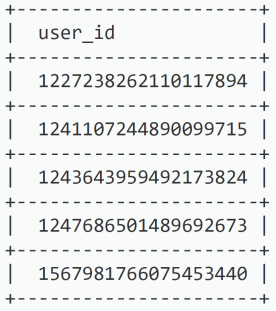
Step 1 - Understand the problem and establish design scope
**Requirements:**
- IDs must be unique. - IDs are numerical values only. - IDs fit into 64-bit. - IDs are ordered by date. - Ability to generate over 10,000 unique IDs per second.
Step 2 - Propose high-level design and get buy-in
Multiple options can be used to generate unique IDs in distributed systems:
- Multi-master replication - Universally unique identifier (UUID) - Ticket server - Twitter snowflake approach
Multi-master replication
As shown in Figure 2, the first approach is multi-master replication.
This approach uses the databases' auto_increment feature. Instead of increasing the next ID by 1, we increase it by k, where k is the number of database servers in use. The next ID to be generated is equal to the previous ID in the same server plus k. This solves some scalability issues because IDs can scale with the number of database servers.
**Drawbacks:** - Hard to scale with multiple data centers. - IDs do not go up with time across multiple servers. - It does not scale well when a server is added or removed.

UUID
A UUID is another easy way to obtain unique IDs. UUID is a 128-bit number used to identify information in computer systems. UUID has a very low probability of collision — "after generating 1 billion UUIDs every second for approximately 100 years would the probability of creating a single duplicate reach 50%" [1].
Example UUID: `09c93e62-50b4-468d-bf8a-c07e1040bfb2`
UUIDs can be generated independently without coordination between servers. In Figure 3, each web server contains its own ID generator and is responsible for generating IDs independently.
**Pros:** - Generating UUID is simple. No coordination between servers is needed so there will not be any synchronization issues. - The system is easy to scale because each web server is responsible for generating IDs they consume.
**Cons:** - IDs are 128 bits long, but our requirement is 64 bits. - IDs do not go up with time. - IDs could be non-numeric.

Ticket Server
Ticket servers are another interesting way to generate unique IDs. Flickr developed ticket servers to generate distributed primary keys [2]. The idea is to use a centralized auto_increment feature in a single database server (Ticket Server).
**Pros:** - Numeric IDs. - It is easy to implement, and it works for small to medium-scale applications.
**Cons:** - Single point of failure. Single ticket server means if the ticket server goes down, all systems that depend on it will face issues. To avoid a single point of failure, we can set up multiple ticket servers. However, this will introduce new challenges such as data synchronization.

Twitter snowflake approach
Twitter's unique ID generation system called "snowflake" [3] is inspiring and can satisfy our requirements. Instead of generating an ID directly, we divide an ID into different sections. Figure 5 shows the layout of a 64-bit ID.
**Sections of a 64-bit Snowflake ID:**
- **Sign bit:** 1 bit. Always 0. Reserved for future uses. Can potentially distinguish between signed and unsigned numbers. - **Timestamp:** 41 bits. Milliseconds since the epoch or custom epoch. Twitter snowflake uses default epoch 1288834974657, equivalent to Nov 04, 2010, 01:42:54 UTC. - **Datacenter ID:** 5 bits → 2^5 = 32 datacenters. - **Machine ID:** 5 bits → 2^5 = 32 machines per datacenter. - **Sequence number:** 12 bits. For every ID generated on that machine/process, the sequence number is incremented by 1. The number is reset to 0 every millisecond.

Step 3 - Design deep dive
We settle on an approach that is based on the Twitter snowflake ID generator (Figure 6).
Datacenter IDs and machine IDs are chosen at startup time, generally fixed once the system is up running. Any changes require careful review since an accidental change in those values can lead to ID conflicts. Timestamp and sequence numbers are generated when the ID generator is running.

Timestamp
The most important 41 bits make up the timestamp section. As timestamps grow with time, IDs are sortable by time. Figure 7 shows an example of how binary representation is converted to UTC.
The maximum timestamp that can be represented in 41 bits is:
``` 2^41 - 1 = 2,199,023,255,551 ms ≈ 69 years ```
This means the ID generator will work for 69 years and having a custom epoch time close to today's date delays the overflow time. After 69 years, we will need a new epoch time or adopt other techniques to migrate IDs.

Sequence number
Sequence number is 12 bits, which gives 2^12 = 4096 combinations. This field is 0 unless more than one ID is generated in a millisecond on the same server. In theory, a machine can support a maximum of 4096 new IDs per millisecond.
Step 4 - Wrap up
We discussed different approaches to design a unique ID generator: multi-master replication, UUID, ticket server, and Twitter snowflake-like unique ID generator. We settle on snowflake as it supports all our use cases and is scalable in a distributed environment.
**Additional talking points:**
- **Clock synchronization.** We assume ID generation servers have the same clock. This assumption might not be true when a server is running on multiple cores. Network Time Protocol is the most popular solution to this problem [4].
- **Section length tuning.** For example, fewer sequence numbers but more timestamp bits are effective for low concurrency and long-term applications.
- **High availability.** Since an ID generator is a mission-critical system, it must be highly available.
Design A URL Shortener
In this chapter, we will tackle an interesting and classic system design interview question: designing a URL shortening service like tinyurl.
Step 1 - Understand the problem and establish design scope
**Basic use cases:** - URL shortening: given a long URL → return a much shorter URL - URL redirecting: given a shorter URL → redirect to the original URL - High availability, scalability, and fault tolerance considerations
**Back of the envelope estimation:** - Write operation: 100 million URLs per day → ~1160 writes/second - Read operation (10:1 ratio): ~11,600 reads/second - 10-year storage: 100M × 365 × 10 = 365 billion records - Average URL length: 100 bytes - Storage over 10 years: 365 billion × 100 bytes = **36.5 TB**
Step 2 - Propose high-level design and get buy-in
API Endpoints
A URL shortener primarily needs two API endpoints:
**URL shortening** — POST request with original long URL: ``` POST api/v1/data/shorten request parameter: {longUrl: longURLString} return: shortURL ```
**URL redirecting** — GET request with short URL: ``` GET api/v1/shortUrl return: longURL for HTTP redirection ```
URL redirecting
Figure 1 shows what happens when you enter a tinyurl onto the browser. Once the server receives a tinyurl request, it changes the short URL to the long URL with 301 redirect.
The detailed communication between clients and servers is shown in Figure 2.
**301 vs 302 redirect:**
- **301 redirect:** The requested URL is "permanently" moved to the long URL. The browser caches the response, and subsequent requests for the same URL will NOT be sent to the URL shortening service — requests go directly to the long URL server. Use when priority is to **reduce server load**.
- **302 redirect:** The URL is "temporarily" moved to the long URL. Subsequent requests for the same URL WILL be sent to the URL shortening service first, then redirected. Use when **analytics** is important (tracks click rate and source).
The most intuitive way to implement URL redirecting is to use hash tables storing `<shortURL, longURL>` pairs.
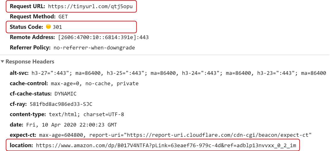
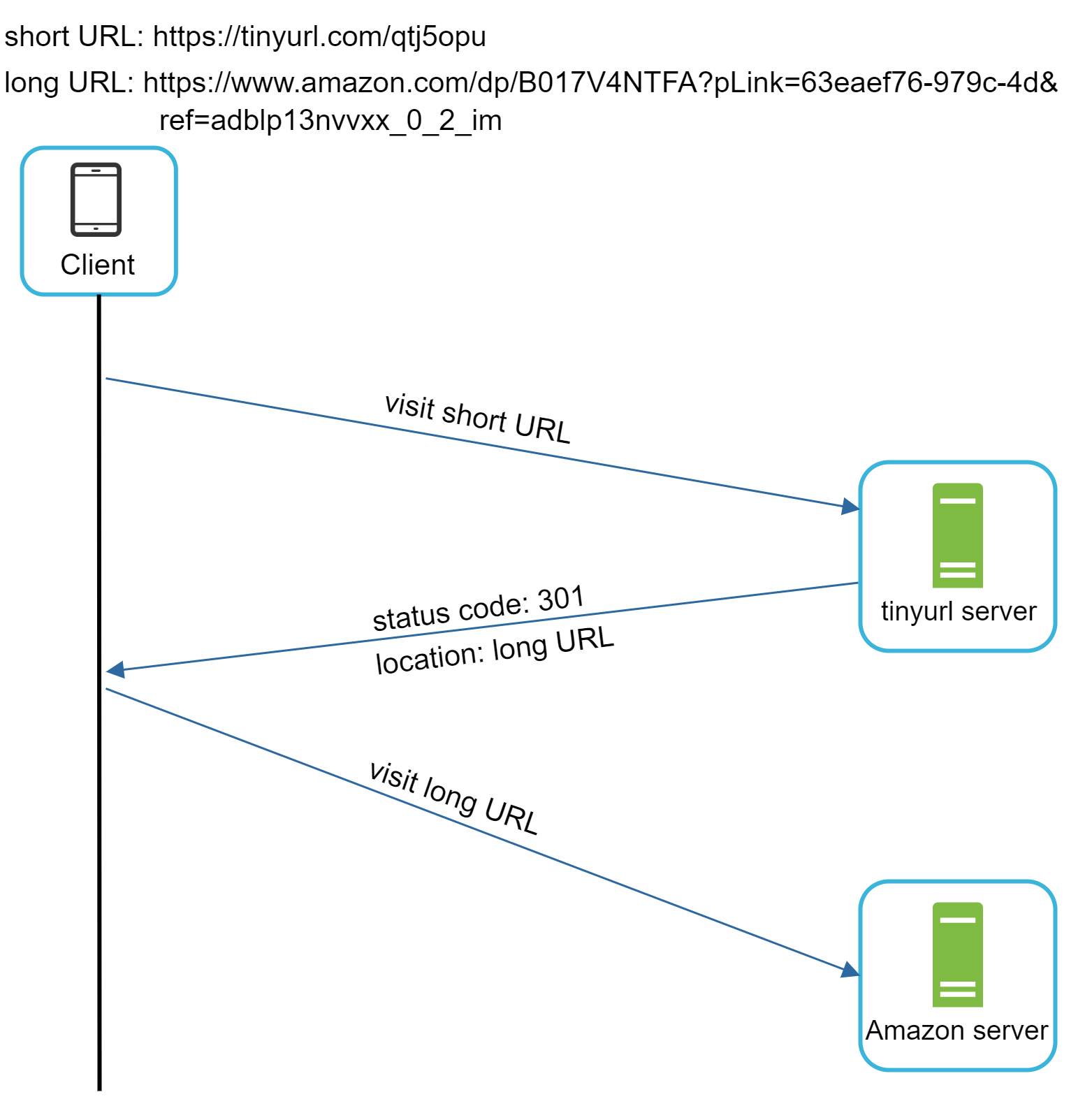
URL shortening
Assume the short URL looks like: `www.tinyurl.com/{hashValue}`. To support URL shortening, we must find a hash function fx that maps a long URL to the hashValue, as shown in Figure 3.
The hash function must satisfy: - Each longURL must be hashed to one hashValue. - Each hashValue can be mapped back to the longURL.

Step 3 - Design deep dive
Data model
In the high-level design, everything is stored in a hash table. This is a good starting point; however, this approach is not feasible for real-world systems as memory resources are limited and expensive. A better option is to store `<shortURL, longURL>` mapping in a relational database. Figure 4 shows a simple database table design with 3 columns: id, shortURL, longURL.
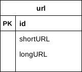
Hash function
Hash function is used to hash a long URL to a short URL (hashValue).
**Hash value length:**
The hashValue consists of characters from [0-9, a-z, A-Z] = 62 possible characters. To find the length n such that 62^n ≥ 365 billion:
| n | Maximal number of URLs | |---|------------------------| | 1 | 62 | | 5 | 916,132,832 | | 6 | 56,800,235,584 | | **7** | **~3.5 trillion** | | 8 | ~218 trillion |
When n = 7, 62^7 ≈ 3.5 trillion — more than enough to hold 365 billion URLs. So **hashValue length = 7**.
Hash + collision resolution
A straightforward solution is to use well-known hash functions like CRC32, MD5, or SHA-1. Even the shortest hash value (from CRC32) is too long. The first approach is to collect the first 7 characters of a hash value; however, this method can lead to hash collisions.
To resolve hash collisions, we recursively append a new predefined string until no more collision is discovered. This process is explained in Figure 5.
This method can eliminate collision; however, it is expensive to query the database to check if a shortURL exists for every request. A **bloom filter** [2] can improve performance — a space-efficient probabilistic technique to test if an element is a member of a set.

Base 62 conversion
Base 62 conversion is another approach commonly used for URL shorteners. Base 62 uses 62 characters for encoding. The mappings are: 0→0, ..., 9→9, 10→a, 11→b, ..., 35→z, 36→A, ..., 61→Z.
Example: convert 11157 (base 10) to base 62:
``` 11157 = 2 × 62² + 55 × 62¹ + 59 × 62⁰ = [2, 55, 59] = [2, T, X] in base 62 ```
Figure 6 shows the conversion process. The short URL would be: `https://tinyurl.com/2TX`
**Comparison of the two approaches:**
| | Hash + collision resolution | Base 62 conversion | |---|---|---| | URL length | Fixed short URL length | Not fixed — grows with the ID | | Unique ID | Does not need a unique ID generator | Depends on a unique ID generator | | Collision | Possible, needs resolution | Not possible (ID is unique) | | Security | Cannot figure out next available short URL | Easy to figure out next short URL (security concern) |

URL shortening deep dive
Base 62 conversion is used in our design. Figure 7 demonstrates the URL shortening flow:
1. longURL is the input. 2. Check if the longURL is already in the database. 3. If yes → fetch the shortURL from the database and return it to the client. 4. If no → generate a new unique ID (primary key) via the unique ID generator. 5. Convert the ID to shortURL with base 62 conversion. 6. Create a new database row with the ID, shortURL, and longURL.
**Concrete example:** - Input: `https://en.wikipedia.org/wiki/Systems_design` - Unique ID generator returns: `2009215674938` - Base 62 conversion: `2009215674938` → `"zn9edcu"` - Save to database: `(2009215674938, "zn9edcu", longURL)`

URL redirecting deep dive
Figure 8 shows the detailed design of URL redirecting. As there are more reads than writes, `<shortURL, longURL>` mapping is stored in a cache to improve performance.
**URL redirecting flow:** 1. A user clicks a short URL link: `https://tinyurl.com/zn9edcu` 2. The load balancer forwards the request to web servers. 3. If a shortURL is already in the cache, return the longURL directly. 4. If a shortURL is not in the cache, fetch the longURL from the database. If it is not in the database, it is likely a user entered an invalid shortURL. 5. The longURL is returned to the user.
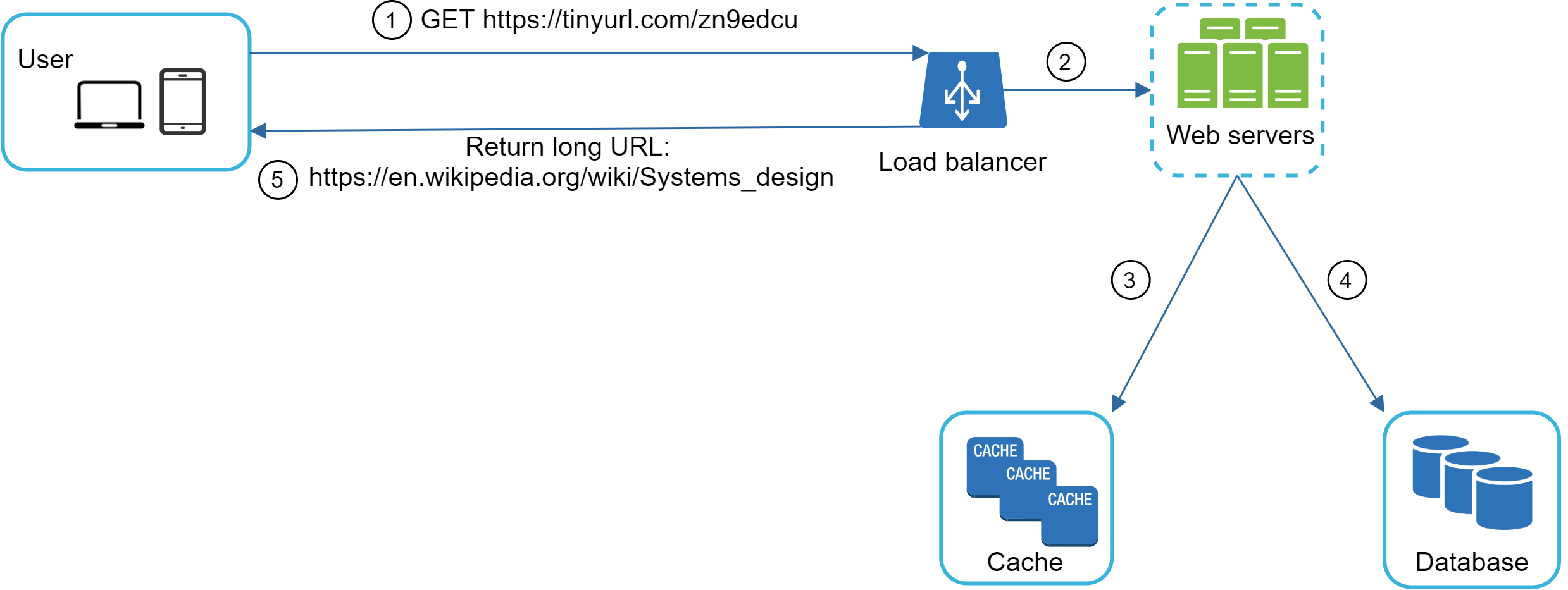
Step 4 - Wrap up
In this chapter, we talked about the API design, data model, hash function, URL shortening, and URL redirecting.
**Additional talking points:**
- **Rate limiter:** A potential security problem — malicious users send overwhelmingly large numbers of URL shortening requests. Rate limiter helps filter out requests based on IP address or other filtering rules. - **Web server scaling:** Since the web tier is stateless, it is easy to scale by adding or removing web servers. - **Database scaling:** Database replication and sharding are common techniques. - **Analytics:** Integrating an analytics solution to answer: how many people click on a link? When do they click? - **Availability, consistency, and reliability:** Core of any large system's success.
Design A Web Crawler
A web crawler is known as a robot or spider. It is widely used by search engines to discover new or updated content on the web. Content can be a web page, an image, a video, a PDF file, etc. A web crawler starts by collecting a few web pages and then follows links on those pages to collect new content. Figure 1 shows a visual example of the crawl process.
**Use cases for web crawlers:** - **Search engine indexing:** Collect web pages to create a local index for search engines. For example, Googlebot is the web crawler behind the Google search engine. - **Web archiving:** Collect information from the web to preserve data for future uses. Examples: US Library of Congress [1], EU web archive [2]. - **Web mining:** Discover useful knowledge from the internet. Top financial firms use crawlers to download shareholder meetings and annual reports. - **Web monitoring:** Monitor copyright and trademark infringements over the Internet. For example, Digimarc [3] utilizes crawlers to discover pirated works.
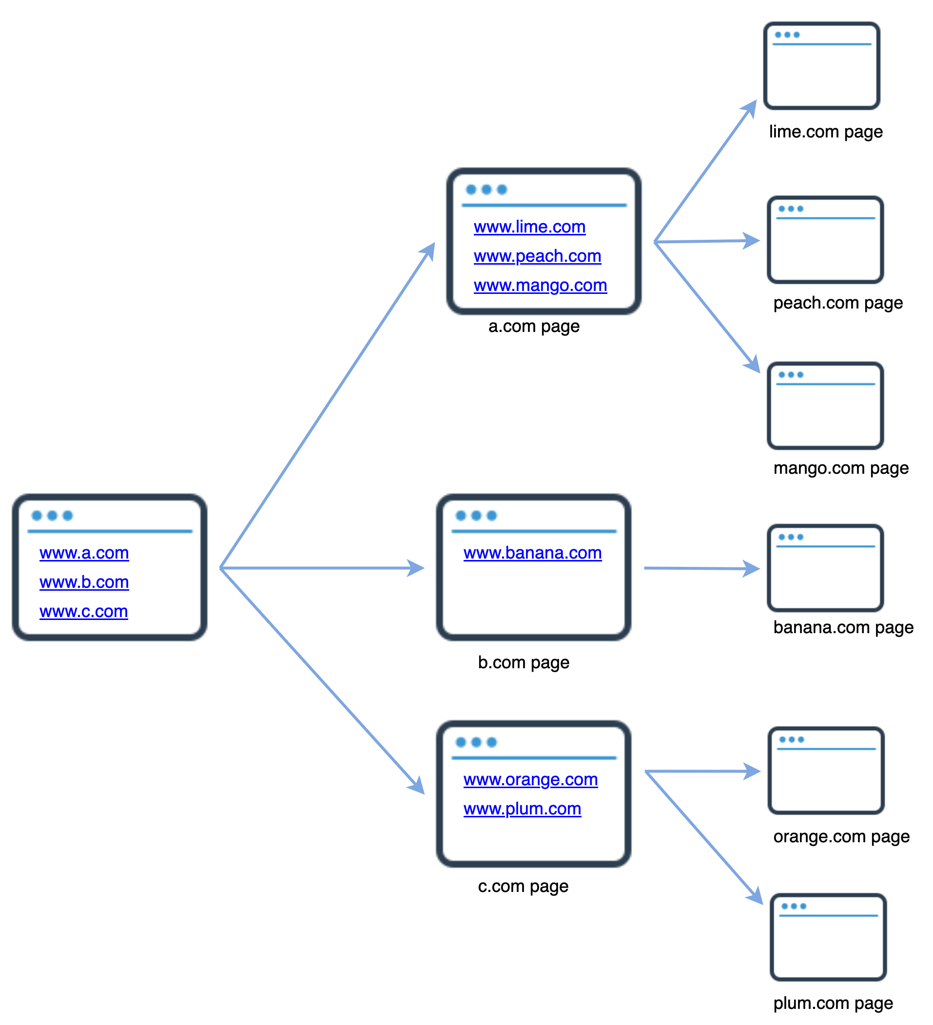
Step 1 - Understand the problem and establish design scope
**Characteristics of a good web crawler:**
- **Scalability:** Web crawling should be extremely efficient using parallelization. - **Robustness:** The crawler must handle bad HTML, unresponsive servers, crashes, malicious links, etc. - **Politeness:** The crawler should not make too many requests to a website within a short time interval. - **Extensibility:** The system is flexible so that minimal changes are needed to support new content types.
**Back of the envelope estimation:** - 1 billion web pages downloaded per month - QPS: 1B / 30 / 24 / 3600 ≈ **400 pages/second** (Peak: 800) - Average web page size: 500 KB - Storage per month: 1B × 500 KB = **500 TB/month** - 5-year storage: 500 TB × 12 × 5 = **30 PB**
Step 2 - Propose high-level design and get buy-in
We propose a high-level design as shown in Figure 2.

Key components
- **Seed URLs:** Starting point for the crawl process. Can be selected based on locality or topic. - **URL Frontier:** Stores URLs to be downloaded (FIFO queue). Ensures politeness, prioritization, and freshness. - **HTML Downloader:** Downloads web pages from the internet via HTTP. - **DNS Resolver:** Translates URLs to IP addresses. - **Content Parser:** Parses and validates downloaded web pages. Separate from crawl server to avoid slowing down crawl. - **Content Seen?:** Detects duplicate content using hash comparison [7]. ~29% of web pages are duplicate [6]. - **Content Storage:** Storage system for HTML content. Popular content in memory; rest on disk. - **URL Extractor:** Parses and extracts links from HTML pages. Converts relative paths to absolute URLs (Figure 3). - **URL Filter:** Excludes certain content types, file extensions, error links, and blacklisted sites. - **URL Seen?:** Data structure (bloom filter + hash table) tracking visited URLs to avoid duplicates. - **URL Storage:** Stores already visited URLs.

Web crawler workflow
Figure 4 shows the workflow step-by-step:
1. Add seed URLs to the URL Frontier. 2. HTML Downloader fetches a list of URLs from URL Frontier. 3. HTML Downloader gets IP addresses from DNS resolver and starts downloading. 4. Content Parser parses HTML pages and checks if pages are malformed. 5. Parsed content is passed to the "Content Seen?" component. 6. "Content Seen" checks if the HTML page is already in storage: - If yes → discard (duplicate content in different URL). - If no → pass to Link Extractor. 7. Link extractor extracts links from HTML pages. 8. Extracted links are passed to the URL filter. 9. Filtered links are passed to the "URL Seen?" component. 10. "URL Seen" checks if a URL is already in storage; if yes, nothing to do. 11. If a URL has not been processed before, add it to the URL Frontier.

Step 3 - Design deep dive
Key topics in depth: DFS vs BFS, URL frontier, HTML Downloader, robustness, extensibility, and problematic content.
DFS vs BFS
The web can be thought of as a directed graph where web pages serve as nodes and hyperlinks as edges. DFS is usually not a good choice because the depth can be very deep.
BFS is commonly used and implemented by a FIFO queue. However, it has two problems:
1. **Politeness problem:** Most links from the same web page are internal links, making the crawler busy processing URLs from the same host. This overwhelms the host server (Figure 5). 2. **Priority problem:** Standard BFS does not take the priority of a URL into consideration. We may want to prioritize URLs according to page ranks, web traffic, update frequency, etc.

URL frontier
URL frontier addresses the BFS problems: politeness, URL prioritization, and freshness.
**Politeness:** Download one page at a time from the same host. A delay is added between two download tasks.
Figure 6 shows the politeness design: - **Queue router:** Ensures each queue (b1, b2, …, bn) only contains URLs from the same host. - **Mapping table:** Maps each host to a queue. - **FIFO queues b1 to bn:** Each queue contains URLs from the same host. - **Queue selector:** Maps each worker thread to a FIFO queue. - **Worker threads 1 to N:** Download web pages one by one from the same host with delay.
**Priority:** We prioritize URLs based on usefulness (PageRank [10], website traffic, update frequency).
Figure 7 shows the priority design: - **Prioritizer:** Takes URLs as input and computes the priorities. - **Queues f1 to fn:** Each queue has an assigned priority. Higher priority queues are selected with higher probability. - **Queue selector:** Randomly choose a queue biased towards higher priority.
Figure 8 shows the complete URL frontier design with front queues (manage prioritization) and back queues (manage politeness).
**Freshness:** Web pages must be periodically recrawled: - Recrawl based on web pages' update history. - Prioritize and recrawl important pages first and more frequently.
**Storage:** Hybrid approach — majority stored on disk, buffers in memory for enqueue/dequeue, periodically flushed to disk.


HTML Downloader
**Robots.txt (Robots Exclusion Protocol):** Standard used by websites to communicate with crawlers. Specifies what pages crawlers are allowed to download. Robots.txt results are cached periodically.
Example from `https://www.amazon.com/robots.txt`: ``` User-agent: Googlebot Disallow: /creatorhub/* Disallow: /rss/people/*/reviews Disallow: /gp/pdp/rss/*/reviews Disallow: /gp/cdp/member-reviews/ Disallow: /gp/aw/cr/ ```
**Performance optimizations:**
1. **Distributed crawl:** Crawl jobs distributed into multiple servers, each running multiple threads. URL space is partitioned into smaller pieces (Figure 9).
2. **Cache DNS Resolver:** DNS resolution can take 10ms–200ms and blocks other threads. Maintain a DNS cache mapping domain names to IP addresses, updated periodically by cron jobs.
3. **Locality:** Distribute crawl servers geographically. Crawl servers closer to website hosts experience faster download times.
4. **Short timeout:** Specify a maximal wait time. If a host does not respond within the predefined time, the crawler stops the job and crawls other pages.

Robustness
- **Consistent hashing:** Distribute loads among downloaders. New downloader servers can be added or removed. - **Save crawl states and data:** Guard against failures. A disrupted crawl can be restarted easily by loading saved states. - **Exception handling:** The crawler must handle exceptions gracefully without crashing. - **Data validation:** Prevent system errors from malformed input.
Extensibility
The crawler can be extended by plugging in new modules as shown in Figure 10:
- **PNG Downloader module:** Plugged in to download PNG files. - **Web Monitor module:** Added to monitor the web and prevent copyright and trademark infringements.

Detect and avoid problematic content
1. **Redundant content:** ~30% of web pages are duplicates. Hashes or checksums detect duplication [11].
2. **Spider traps:** Web pages that cause a crawler in an infinite loop (e.g., infinite deep directory structures). Avoided by setting a maximal URL length. Websites with spider traps are identifiable by unusually large numbers of discovered web pages.
3. **Data noise:** Advertisements, code snippets, spam URLs, etc. should be excluded if possible.
Step 4 - Wrap up
We discussed the characteristics of a good crawler: scalability, politeness, extensibility, and robustness.
**Additional talking points:**
- **Server-side rendering:** Websites using JavaScript/AJAX generate links dynamically. Perform server-side rendering (dynamic rendering) first before parsing [12]. - **Filter out unwanted pages:** Anti-spam component to filter out low quality and spam pages [13] [14]. - **Database replication and sharding:** Improve data layer availability, scalability, and reliability. - **Horizontal scaling:** Hundreds or thousands of servers needed for large-scale crawl. Keep servers stateless. - **Availability, consistency, and reliability:** Core of any large system's success. - **Analytics:** Collecting and analyzing data is important for fine-tuning.
Design A Notification System
A notification system is one of the most popular features of many applications. It alerts users with important information like breaking news, product updates, events, offerings, etc. It has become an indispensable part of our daily life. In this chapter, we design a notification system.
A notification is more than just mobile push notification. Three types of notification formats are: mobile push notification, SMS message, and Email. Figure 1 shows examples of each.

Step 1 - Understand the problem and establish design scope
**Requirements:**
- Push notifications, SMS messages, and emails are all supported. - Soft real-time system. Notifications should be delivered as soon as possible; slight delay is acceptable under high load. - Supported devices: iOS devices, android devices, laptop/desktop. - Notifications can be triggered by client applications or scheduled on the server-side. - Users can opt-out of receiving notifications. - 10 million mobile push notifications, 1 million SMS messages, 5 million emails per day.
Step 2 - Propose high-level design and get buy-in
This section presents the high-level designs that support various notification types: iOS push notification, Android push notification, SMS message, and Email.
Different types of notifications
**iOS push notification:**
Figure 2 shows how iOS push notification works.
To send an iOS push notification, three components are needed: - **Provider:** Builds and sends notification requests to Apple Push Notification Service (APNs). A notification request includes a device token and payload. Device token is a unique identifier used for sending push notifications. Payload is a JSON dictionary with notification details. - **APNs:** A remote service provided by Apple to propagate push notifications to iOS devices. - **iOS Device:** The end client, which receives push notifications.
**Android push notification:**
Android adopts a similar notification flow. Instead of using APNs, Firebase Cloud Messaging (FCM) is commonly used to send push notifications to Android devices (Figure 3).
**SMS message:**
For SMS messages, third party SMS services like Twilio [1], Nexmo [2], and many others are used (Figure 4).
**Email:**
Although companies can set up their own email servers, many use commercial email services. Figure 5 shows the email notification flow. Sendgrid [3] and Mailchimp [4] are among the most popular email services, which offer a better delivery rate and analytics.
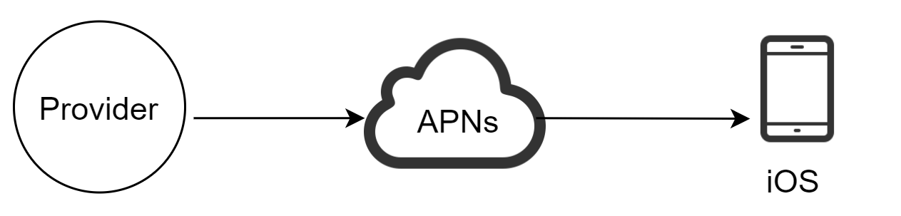
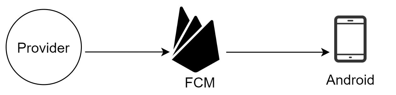
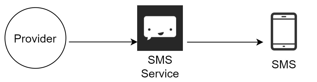
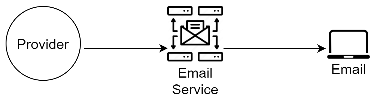
Contact info gathering flow
To send notifications, we need to gather mobile device tokens, phone numbers, or email addresses. As shown in Figure 6, when a user installs our app or signs up for the first time, API servers collect user contact info and store it in the database.
Figure 7 shows simplified database tables for storing contact info. The email address and phone number are stored in the user table. Device tokens are stored in the device table. A user can have multiple devices, indicating push notifications can be sent to all devices.
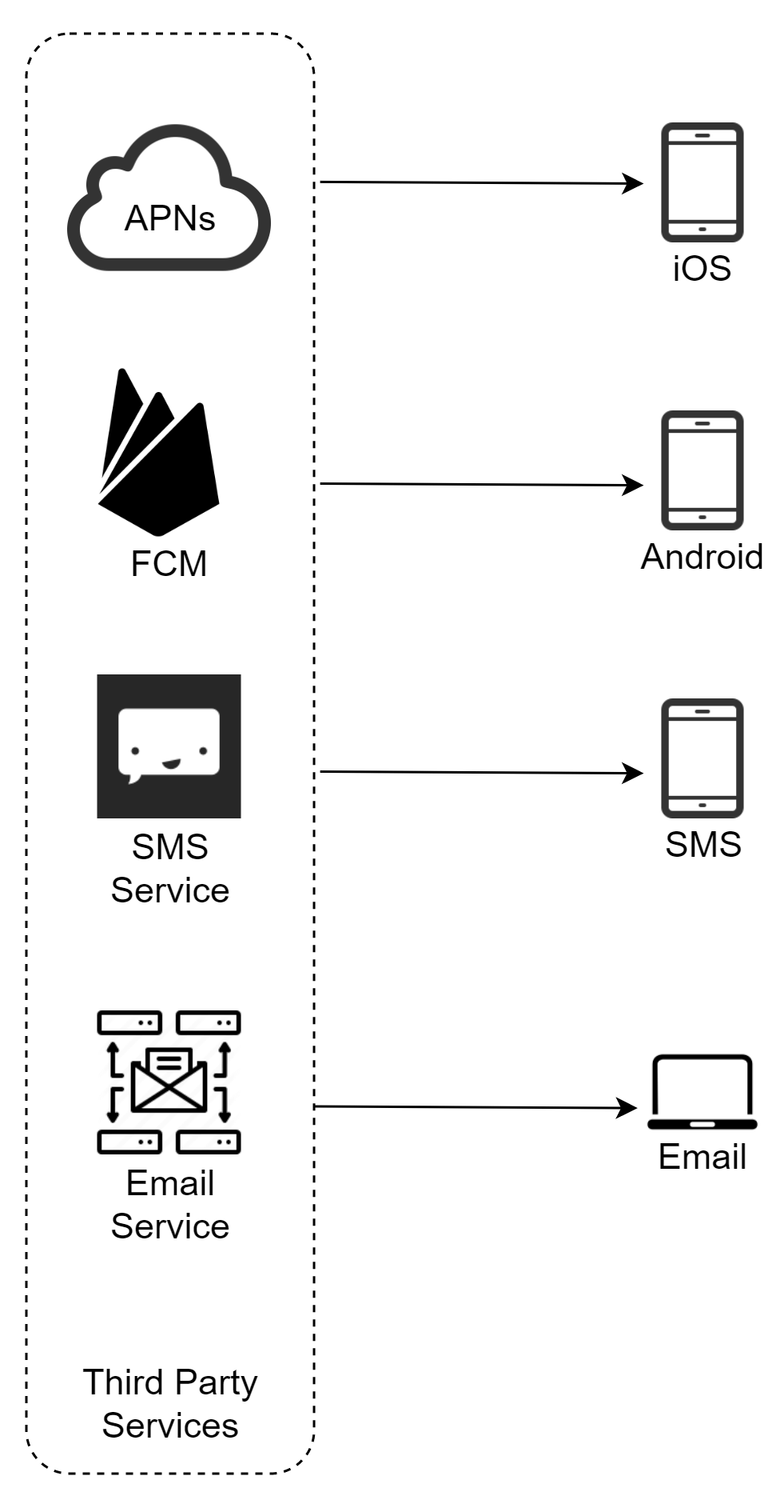
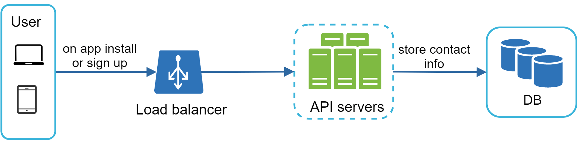
Notification sending/receiving flow
Figure 8 shows the database tables for notification system: user, device, notification tables.
**High-level design (Figure 9):**
- **Service 1 to N:** A service can be a micro-service, a cron job, or a distributed system that triggers notification sending events. - **Notification system:** The notification system is the centerpiece of sending/receiving notifications. Starting with something simple, only one notification server is used. It provides APIs for services 1 to N, and builds notification payloads for third party services. - **Third-party services:** Responsible for delivering notifications to users. Integration with third-party services needs careful consideration. A good extensibility is important as we might want to switch services later. - **iOS, Android, SMS, Email:** Users receive notifications on their devices.
**Problems with the initial design:** - Single point of failure (SPOF): A single notification server means any issue will result in failure of the entire system. - Hard to scale: The notification system handles everything related to push notifications in one server. - Performance bottleneck: Processing and sending notifications can be resource intensive. Handling everything in one system can result in the system overload.
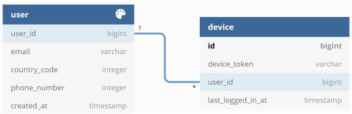

High-level design (improved)
Figure 10 shows the improved high-level design.
- **Move the database and cache out of the notification server.** - **Add more notification servers and set up automatic horizontal scaling.** - **Introduce message queues to decouple the system components.**
Components: - **Service 1 to N:** They represent different services that send notifications via APIs provided by notification servers. - **Notification servers:** They provide the following functionalities: - Provide APIs for services to send notifications. - Basic validations to verify emails, phone numbers, etc. - Query the database or cache to fetch data needed to render notifications. - Put notification data to message queues for parallel processing. - **Cache:** User info, device info, notification templates are cached. - **DB:** Store data about user, notification, settings, etc. - **Message queues:** Serve as buffers when high volumes of notifications are to be sent. Each notification type is assigned a separate message queue. - **Workers:** Pull notification events from message queues and send to corresponding third-party services. - **Third-party services, iOS, Android, SMS, Email:** Same as the initial design.
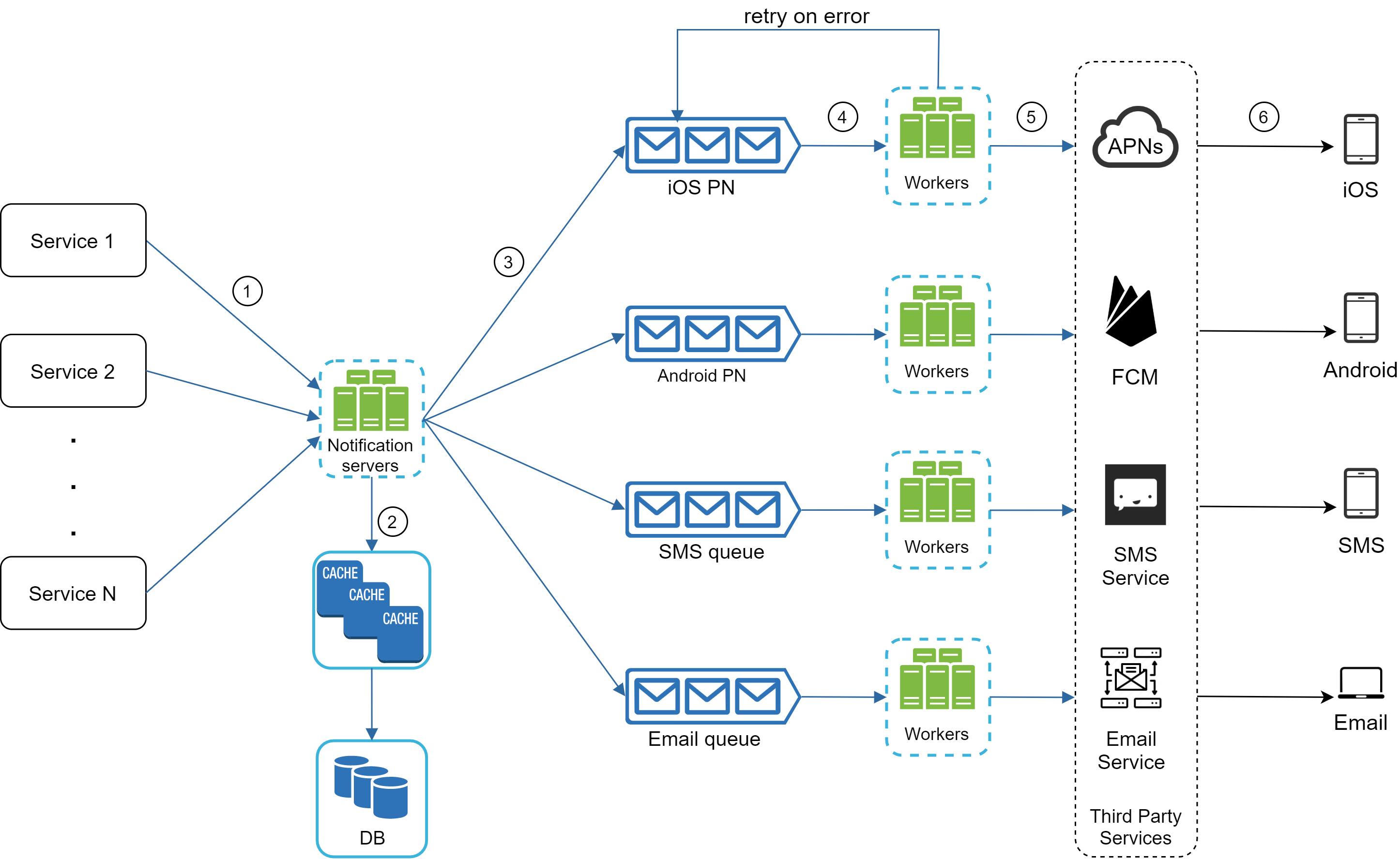
Step 3 - Design deep dive
Key topics: reliability, additional components and considerations, updated design.
Reliability
**How to prevent data loss?**
Notifications can usually not be lost. A notification log database is used for data persistence (Figure 11). The notification log includes data fields such as notification id, type, user id, channel, status, etc.
**Will recipients receive a notification exactly once?**
The short answer is no. Although notification is delivered exactly once most of the time, the distributed nature could result in duplicate notifications. To reduce the duplication occurrence, we introduce a dedupe mechanism and handle each failure case carefully: - When a notification event first arrives, we check if it is seen before by checking the event ID. - If it is seen before, it is discarded. Otherwise, we will send out the notification.

Additional components and considerations
**Notification template:** A large notification system sends out millions of notifications per day, and many notifications follow a similar format. Notification templates are introduced to avoid building every notification from scratch. A notification template is a preformatted notification to create your unique notification by customizing parameters, styling, tracking links, etc.
**Notification setting:** Users are generally provided fine-grained control over notification settings. Before any notification is sent to a user, we first check if a user has opted-in to receive this type of notification.
**Rate limiting:** To avoid overwhelming users with too many notifications, we can limit the number of notifications a user can receive. This is important because receivers could turn off notifications altogether if we send too often.
**Retry mechanism:** When a third-party service fails to send a notification, the notification will be added to the message queue for retrying. If the problem persists, an alert will be sent out to developers.
**Security in push notifications:** For iOS or Android apps, appKey and appSecret are used to secure push notification APIs. Only authenticated or verified clients are allowed to send push notifications using our APIs.
**Monitor queued notifications:** A key metric to monitor is the total number of queued notifications. If the number is large, the notification events are not processed fast enough by workers. More workers are added to handle the situation (Figure 12).
**Event tracking:** Notification metrics, such as open rate, click rate, and engagement are important for understanding customer behaviors. Analytics service implements events tracking. Integration between the notification system and the analytics service is usually required (Figure 13).

Updated design
Putting everything together, Figure 14 shows the updated notification system design, incorporating: notification log, notification settings, rate limiting, retry mechanism, security, monitoring, and event tracking.
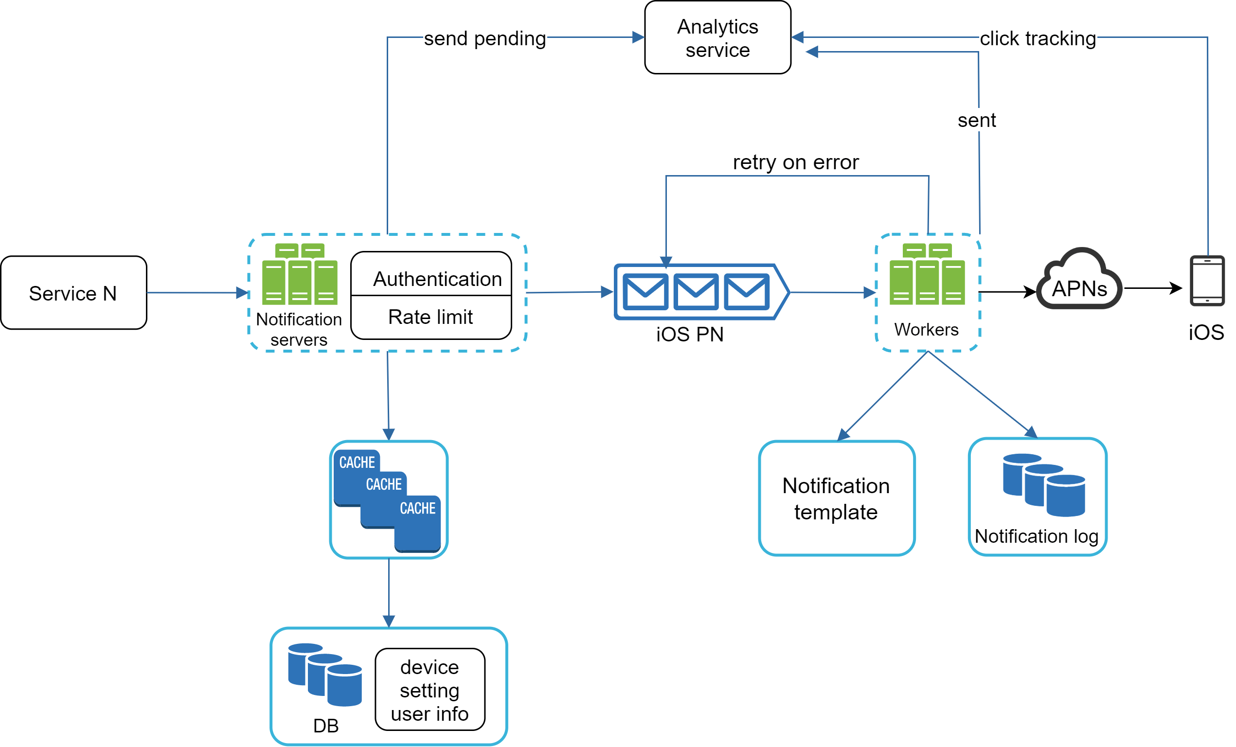
Step 4 - Wrap up
Notifications are indispensable because they keep us posted with important information. We described the design of a notification system that supports push notification, SMS, and email.
We adopted message queues to decouple system components.
Other topics worth discussing:
- **Reliability:** Robust retry mechanism to minimize failure rate. - **Security:** AppKey/appSecret pair to ensure only verified clients send notifications. - **Tracking and monitoring:** Implement event tracking and monitoring to ensure system health. - **Respect user settings:** Users may opt-out of receiving notifications. Our system respects user settings. - **Rate limiting:** Limit frequency of notifications users can receive.
Design A News Feed System
In this chapter, you are asked to design a news feed system. What is news feed? According to the Facebook help page, "News feed is the constantly updating list of stories in the middle of your home page. News Feed includes status updates, photos, videos, links, app activity, and likes from people, pages, and groups that you follow on Facebook" [1]. This is a popular interview question. Similar questions commonly asked are to: design Facebook news feed, Instagram feed, Twitter timeline, etc.
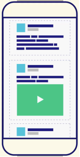
Step 1 - Understand the problem and establish design scope
**Requirements:**
- Both mobile app and web app. - A user can publish a post and see her friends' posts on the news feed page. - News feed is sorted by reverse chronological order. - A user can have up to 5000 friends. - 10 million DAU. - Feed can contain media files, including both images and videos.
Step 2 - Propose high-level design and get buy-in
The design is divided into two flows: feed publishing and news feed building.
- **Feed publishing:** when a user publishes a post, corresponding data is written into cache and database. A post is populated to her friends' news feed. - **Newsfeed building:** for simplicity, the news feed is built by aggregating friends' posts in reverse chronological order.
**Newsfeed APIs:**
The news feed APIs are HTTP based. Two most important APIs:
**Feed publishing API:** ``` POST /v1/me/feed Params: content: text of the post auth_token: authenticate API requests ```
**Newsfeed retrieval API:** ``` GET /v1/me/feed Params: auth_token: authenticate API requests ```
Feed publishing
Figure 2 shows the high-level design of the feed publishing flow.
- **User:** makes a post through API `/v1/me/feed?content=Hello&auth_token={auth_token}` - **Load balancer:** distribute traffic to web servers. - **Web servers:** redirect traffic to different internal services. - **Post service:** persist post in the database and cache. - **Fanout service:** push new content to friends' news feed. Newsfeed data is stored in the cache for fast retrieval. - **Notification service:** inform friends that new content is available and send out push notifications.
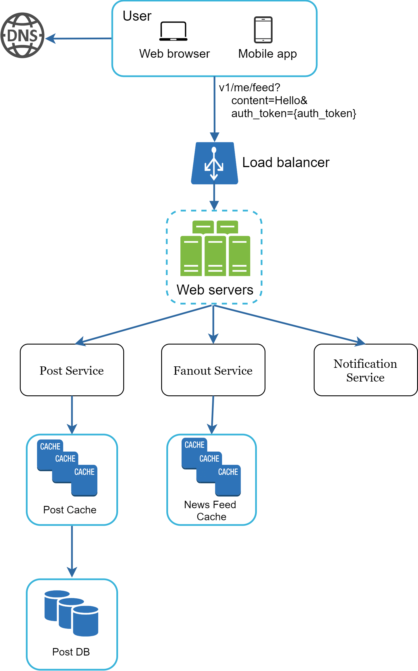
Newsfeed building
Figure 3 shows the high-level design of the newsfeed building flow.
- **User:** sends a request to retrieve her news feed: `/v1/me/feed` - **Load balancer:** redirects traffic to web servers. - **Web servers:** route requests to newsfeed service. - **Newsfeed service:** fetches news feed from the cache. - **Newsfeed cache:** stores news feed IDs needed to render the news feed.
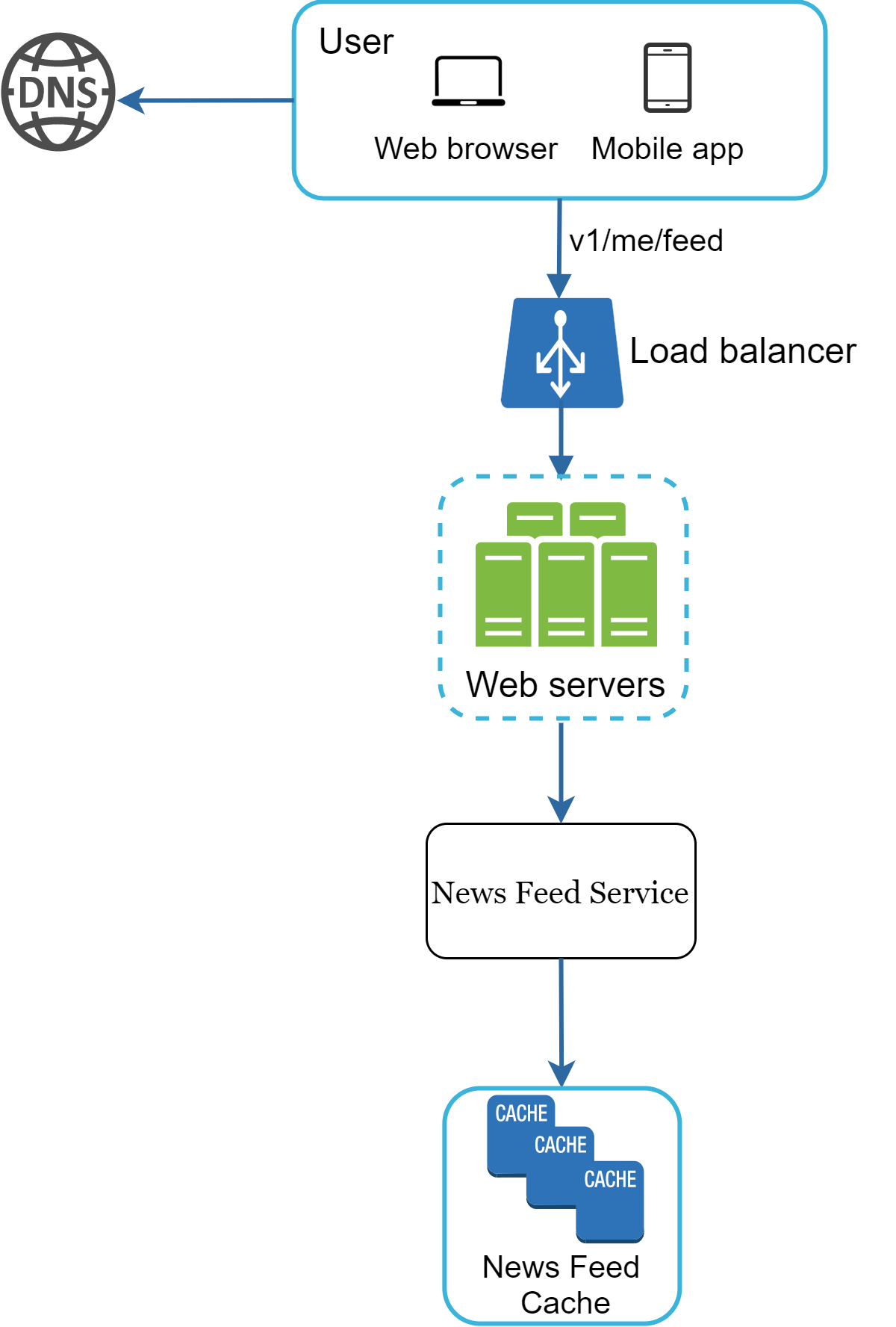
Step 3 - Design deep dive
The high-level design briefly covered two flows: feed publishing and news feed building. Here, we discuss those topics in more depth.
Feed publishing deep dive
Figure 4 outlines the detailed design for feed publishing. We focus on two components: web servers and fanout service.
**Web servers:** Besides communicating with clients, web servers enforce authentication and rate-limiting. Only users signed in with valid auth_token are allowed to make posts. The system limits the number of posts a user can make within a certain period, vital to prevent spam and abusive content.
**Fanout service:** Fanout is the process of delivering a post to all friends. Two types of fanout models:
**Fanout on write (push model):** News feed is pre-computed during write time. A new post is delivered to friends' cache immediately after it is published. - *Pros:* News feed generated in real-time; fast fetching since pre-computed. - *Cons:* Slow for users with many friends (hotkey problem); wastes resources for inactive users.
**Fanout on read (pull model):** News feed generated during read time. Recent posts pulled when a user loads her home page. - *Pros:* No wasted resources for inactive users; no hotkey problem. - *Cons:* Fetching news feed is slow (not pre-computed).
**Hybrid approach:** Use push model for majority of users. For celebrities or users with many friends/followers, let followers pull news content on-demand. Consistent hashing helps mitigate the hotkey problem.
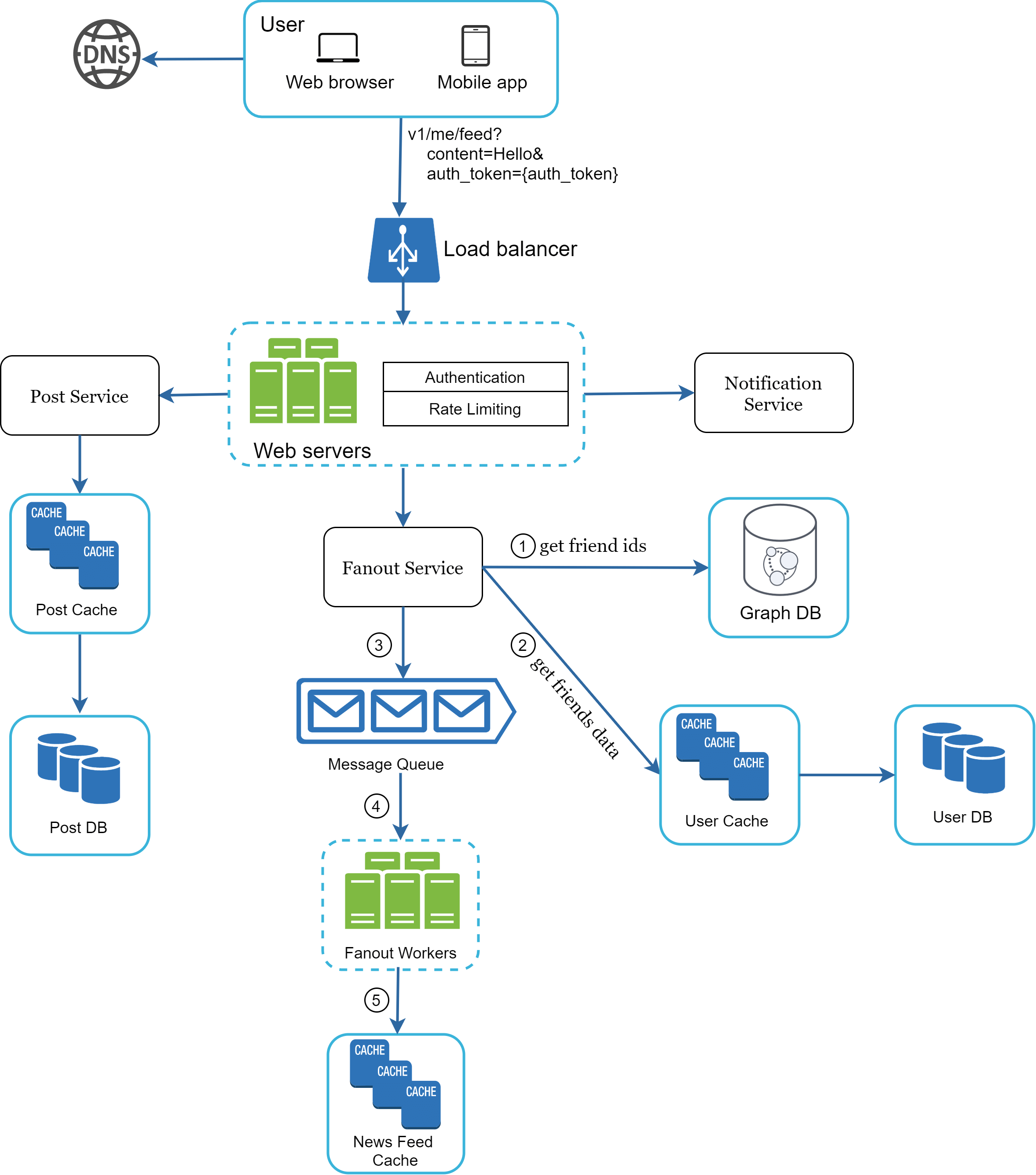
Fanout service
Figure 5 shows the detailed fanout service flow:
1. Fetch friend IDs from the graph database. Graph databases are suited for managing friend relationships and friend recommendations. 2. Get friends info from the user cache. Filter out friends based on user settings (muted users, restricted posts). 3. Send friends list and new post ID to the message queue. 4. Fanout workers fetch data from the message queue and store news feed data in the news feed cache as a `<post_id, user_id>` mapping table. Only IDs are stored to keep memory size small. A configurable limit is set. 5. Store `<post_id, user_id>` in news feed cache (Figure 6).
**Figure 6 — News feed cache table:**
| post_id | user_id | |---------|---------|

Newsfeed retrieval deep dive
Figure 7 illustrates the detailed design for news feed retrieval. Media content (images, videos) are stored in CDN for fast retrieval.
1. User sends request: `/v1/me/feed` 2. Load balancer redistributes requests to web servers. 3. Web servers call the news feed service to fetch news feeds. 4. News feed service gets a list of post IDs from the news feed cache. 5. News feed service fetches complete user and post objects from caches (user cache and post cache) to construct the fully hydrated news feed. 6. The fully hydrated news feed is returned in JSON format to the client for rendering.
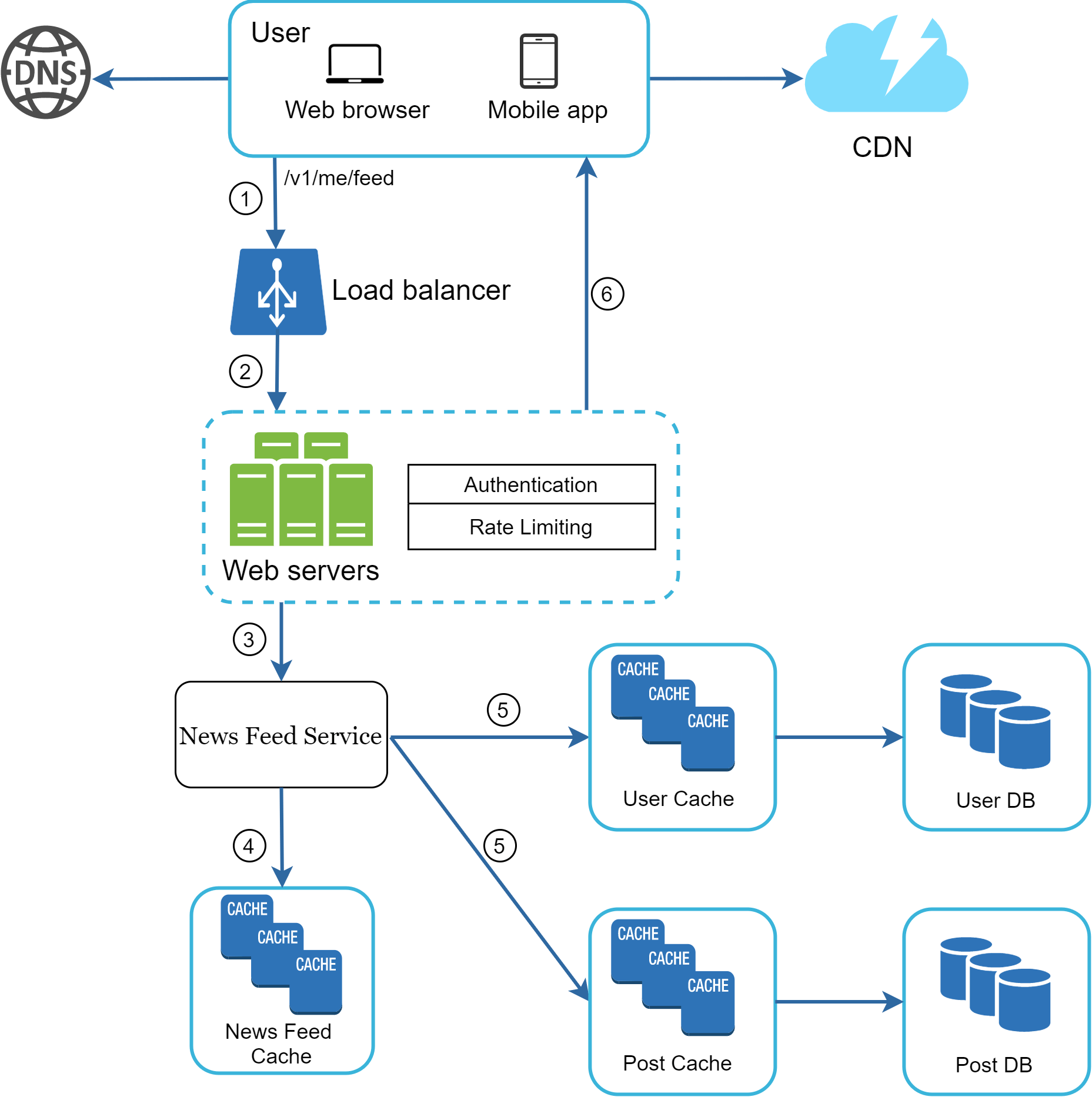
Cache architecture
Cache is extremely important for a news feed system. The cache tier is divided into 5 layers (Figure 8):
- **News Feed:** Stores IDs of news feeds. - **Content:** Stores every post data. Popular content stored in hot cache. - **Social Graph:** Stores user relationship data. - **Action:** Stores info about whether a user liked a post, replied, or took other actions. - **Counters:** Stores counters for like, reply, follower, following, etc.

Step 4 - Wrap up
We designed a news feed system with two flows: feed publishing and news feed retrieval.
**Scaling the database:** - Vertical scaling vs Horizontal scaling - SQL vs NoSQL - Master-slave replication - Read replicas - Consistency models - Database sharding
**Other talking points:** - Keep web tier stateless - Cache data as much as you can - Support multiple data centers - Loosely coupled components with message queues - Monitor key metrics (QPS during peak hours, latency while users refreshing news feed)
Design A Chat System
In this chapter we explore the design of a chat system. Almost everyone uses a chat app. A chat app performs different functions for different people — one-on-one chat apps like Facebook Messenger, WeChat, WhatsApp; office chat apps like Slack; or game chat apps like Discord.
Step 1 - Understand the problem and establish design scope
**Requirements:**
- Support both 1 on 1 and group chat. - Both mobile app and web app. - 50 million daily active users (DAU). - Group chat maximum of 100 people. - Features: 1 on 1 chat, group chat, online indicator. Text messages only. - Message size limit: less than 100,000 characters. - End-to-end encryption: not required for now. - Chat history stored forever.
**Focus features:** - One-on-one chat with low delivery latency - Small group chat (max 100 people) - Online presence - Multiple device support (same account on multiple devices) - Push notifications
Step 2 - Propose high-level design and get buy-in
Clients do not communicate directly with each other. Each client connects to a chat service. The chat service must: - Receive messages from other clients. - Find the right recipients for each message and relay the message. - If a recipient is not online, hold the messages until she is online.
Figure 2 shows the relationships between clients (sender and receiver) and the chat service.

Polling
As shown in Figure 3, polling is a technique where the client periodically asks the server if there are messages available. Depending on polling frequency, polling could be costly — it consumes precious server resources to answer a question that offers "no" as an answer most of the time.

Long polling
Because polling is inefficient, the next progression is long polling (Figure 4). In long polling, a client holds the connection open until there are new messages available or a timeout threshold is reached. Once new messages are received, it immediately sends another request.
**Drawbacks:** - Sender and receiver may not connect to the same chat server (HTTP servers are stateless). - A server has no good way to tell if a client is disconnected. - Inefficient for users who do not chat much — long polling still makes periodic connections after timeouts.

WebSocket
WebSocket is the most common solution for sending asynchronous updates from server to client (Figure 5). WebSocket connection is initiated by the client. It is bi-directional and persistent. It starts as an HTTP connection and is "upgraded" via a well-defined handshake. WebSocket connections work even if a firewall is in place because they use port 80 or 443.
Figure 6 shows WebSocket (ws) used for both sender and receiver sides. By using WebSocket for both, the design is simplified and implementation is more straightforward. Since WebSocket connections are persistent, efficient connection management is critical on the server-side.

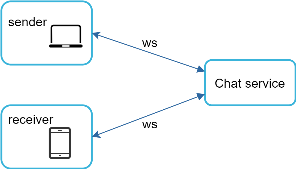
High-level design
WebSocket is chosen as the main communication protocol for bidirectional communication. However, most other features (sign up, login, user profile) use traditional request/response HTTP.
As shown in Figure 7, the chat system is broken down into three major categories: stateless services, stateful services, and third-party integration.
- **Stateless Services:** Handle login, signup, user profile, etc. Sit behind a load balancer. Service discovery gives clients a list of DNS host names of chat servers. - **Stateful Service:** The chat service. Each client maintains a persistent WebSocket connection to a chat server. - **Third-party integration:** Push notification is the most important integration — informs users when new messages arrive even when the app is not running.
Figure 8 shows the adjusted high-level design: - Client maintains a persistent WebSocket connection to a chat server for real-time messaging. - Chat servers facilitate message sending/receiving. - Presence servers manage online/offline status. - API servers handle user login, signup, change profile, etc. - Notification servers send push notifications. - Key-value store stores chat history.
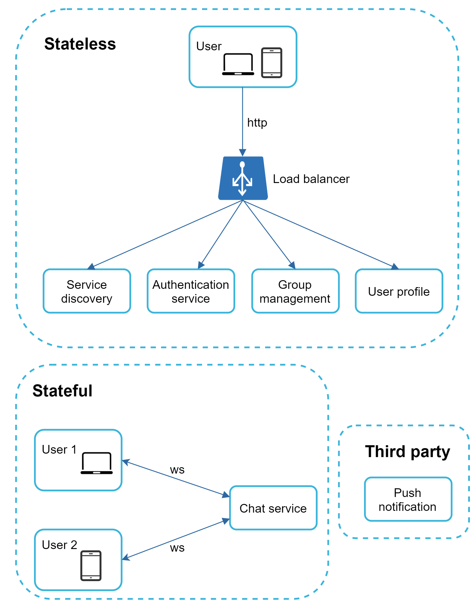
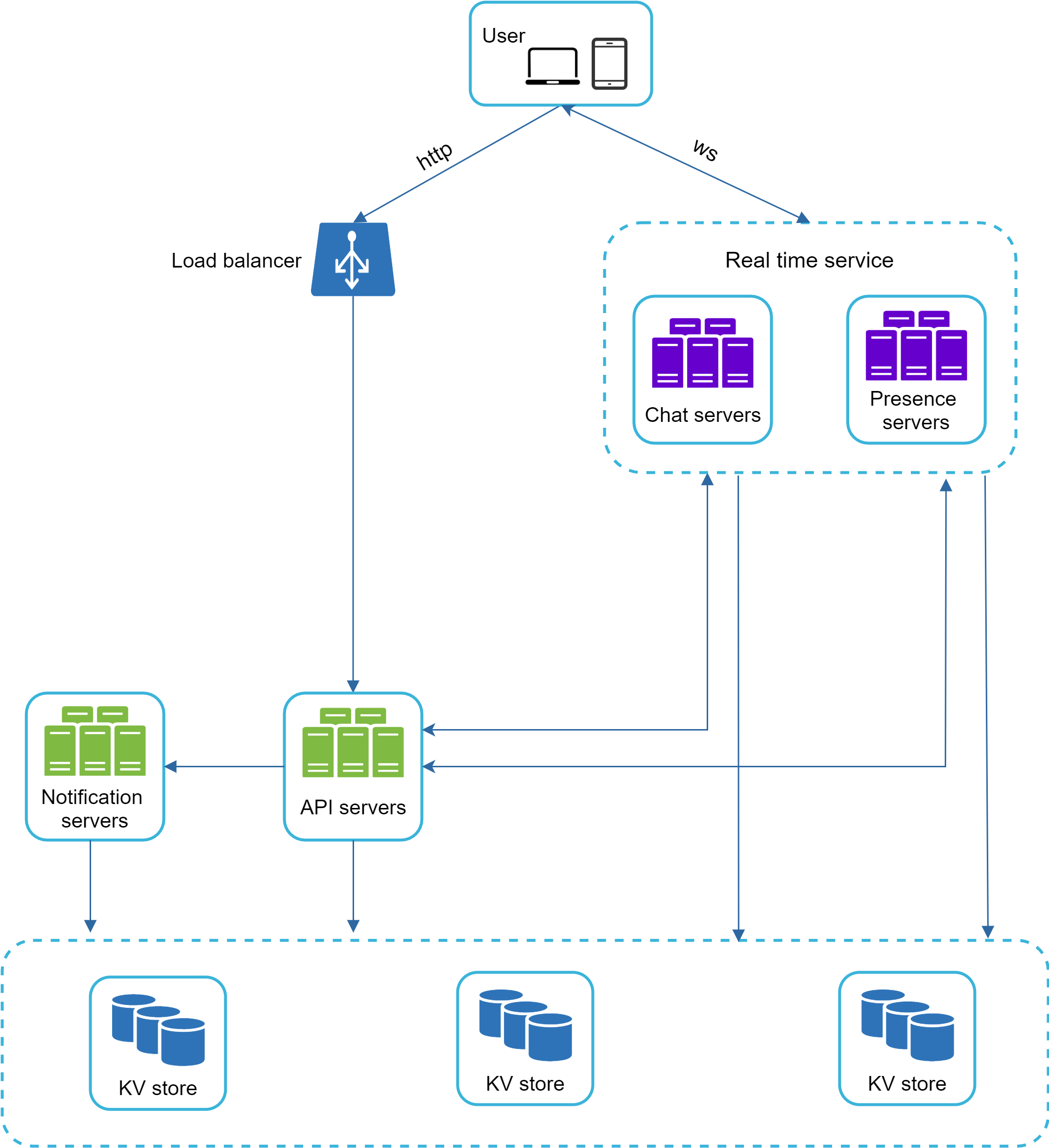
Storage
Two types of data exist in a chat system:
1. **Generic data** (user profile, settings, friends list): Stored in relational databases. Replication and sharding for availability and scalability.
2. **Chat history data**: Key characteristics: - Enormous amount of data (Facebook Messenger and WhatsApp process 60 billion messages/day [2]). - Only recent chats accessed frequently. - Random access needed for search, mentions, jumping to specific messages. - Read/write ratio is about 1:1 for 1-on-1 chat.
**Key-value stores are recommended because:** - Allow easy horizontal scaling. - Provide very low latency to access data. - Relational databases do not handle long tail of data well. - Proven in production: Facebook Messenger uses HBase [4], Discord uses Cassandra [5].
Data models
**Message table for 1 on 1 chat (Figure 9):** Primary key is `message_id`, which helps decide message sequence. We cannot rely on `created_at` because two messages can be created at the same time.
**Message table for group chat (Figure 10):** Composite primary key is `(channel_id, message_id)`. `channel_id` is the partition key because all queries in a group chat operate in a channel.
**Message ID generation:** Must satisfy: - IDs must be unique. - IDs should be sortable by time (new rows have higher IDs).
Approaches: - `auto_increment` in MySQL — not available in NoSQL. - Global 64-bit sequence number generator like Snowflake (see Chapter 8). - Local sequence number generator — IDs unique within a group/channel only.
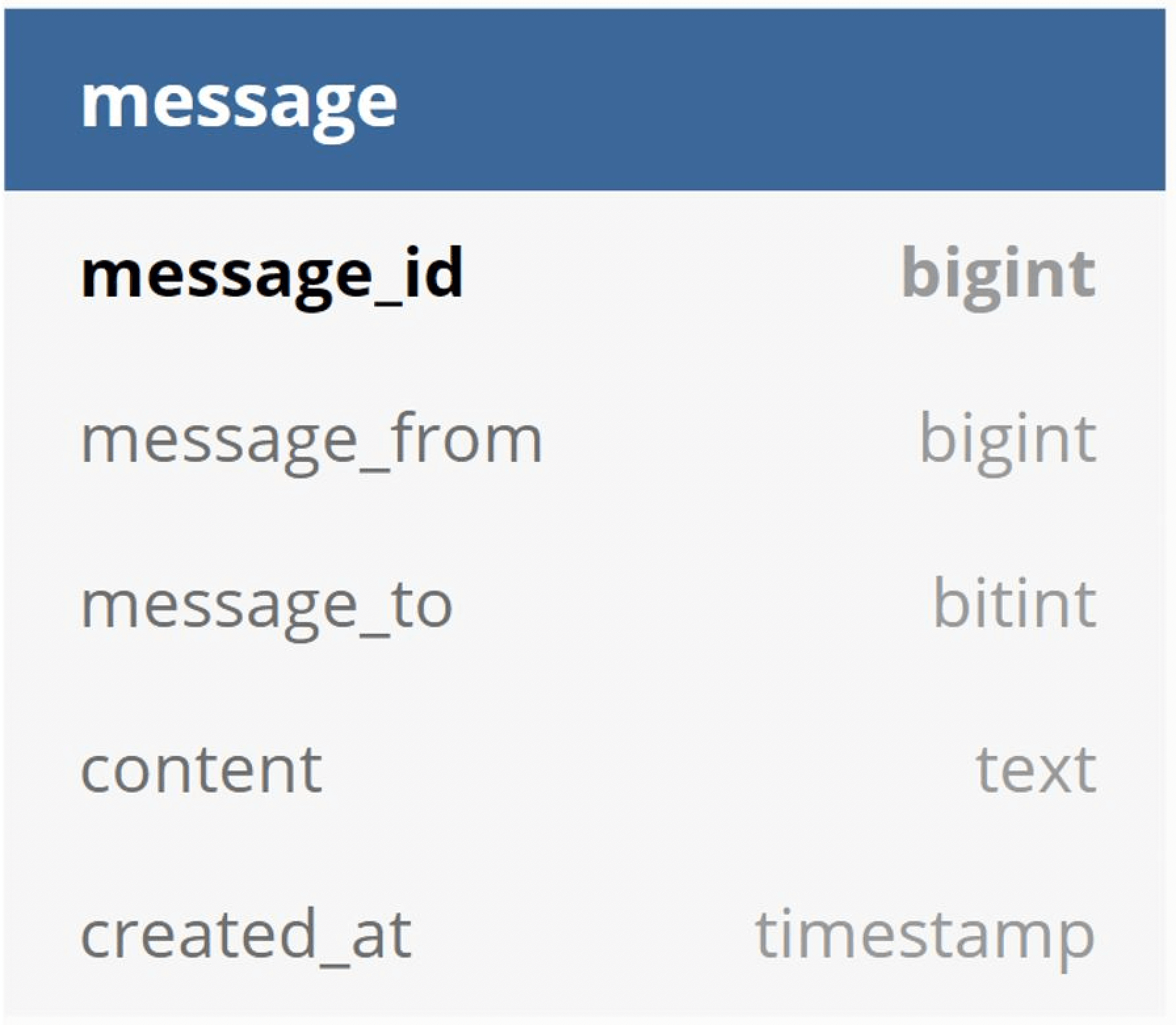
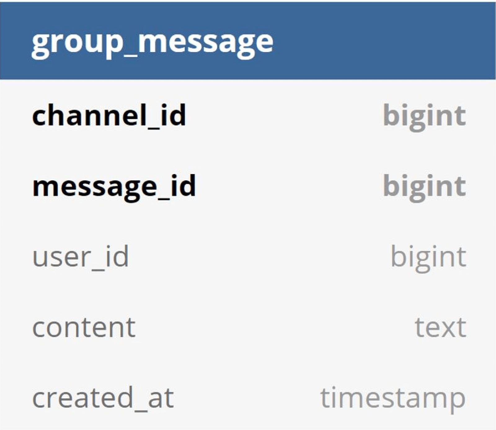
Step 3 - Design deep dive
Key deep dive topics: service discovery, messaging flows, and online/offline indicators.
Service discovery
Service discovery recommends the best chat server for a client based on geographical location, server capacity, etc. Apache Zookeeper [7] is a popular open-source solution.
Figure 11 shows how Zookeeper works: 1. User A tries to log in. 2. Load balancer sends login request to API servers. 3. After authentication, service discovery finds the best chat server for User A (server 2 is chosen). 4. User A connects to chat server 2 through WebSocket.
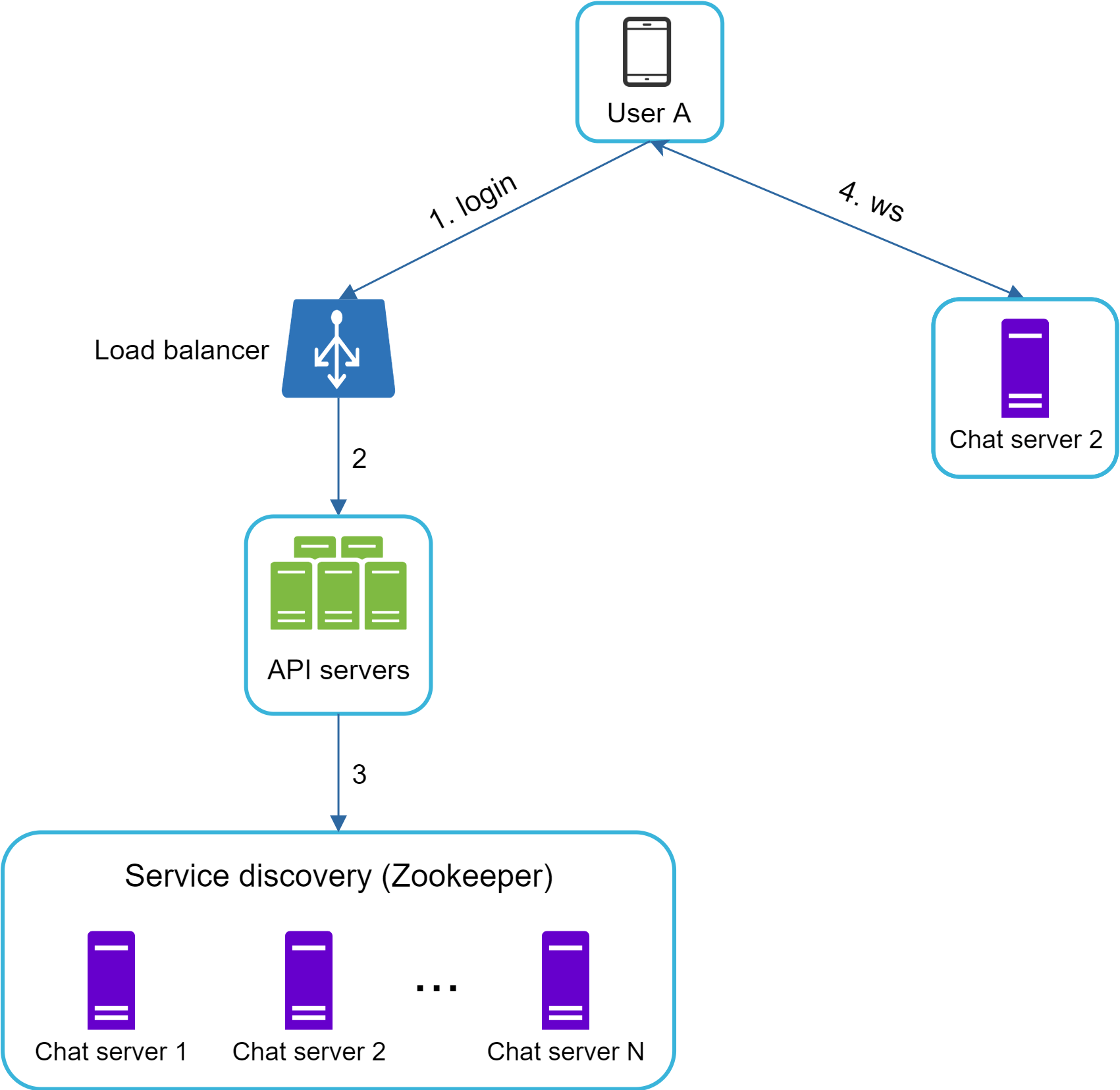
1 on 1 chat flow
Figure 12 explains what happens when User A sends a message to User B:
1. User A sends a chat message to Chat server 1. 2. Chat server 1 obtains a message ID from the ID generator. 3. Chat server 1 sends the message to the message sync queue. 4. The message is stored in a key-value store. 5a. If User B is online, the message is forwarded to Chat server 2 where User B is connected. 5b. If User B is offline, a push notification is sent from push notification (PN) servers. 6. Chat server 2 forwards the message to User B via persistent WebSocket connection.
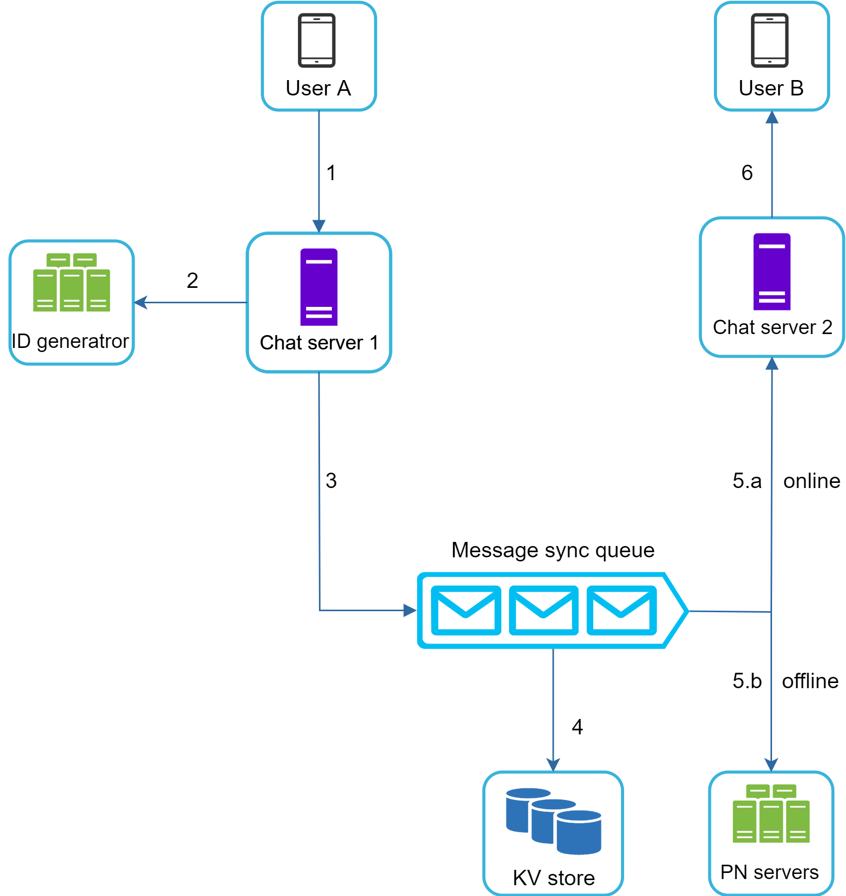
Message synchronization across multiple devices
Figure 13 shows message synchronization across devices. Each device maintains a variable `cur_max_message_id`, which tracks the latest message ID on the device.
Messages are considered new when: - The recipient ID equals the currently logged-in user ID. - Message ID in the key-value store is larger than `cur_max_message_id`.
With distinct `cur_max_message_id` on each device, each device can independently get new messages from the KV store.
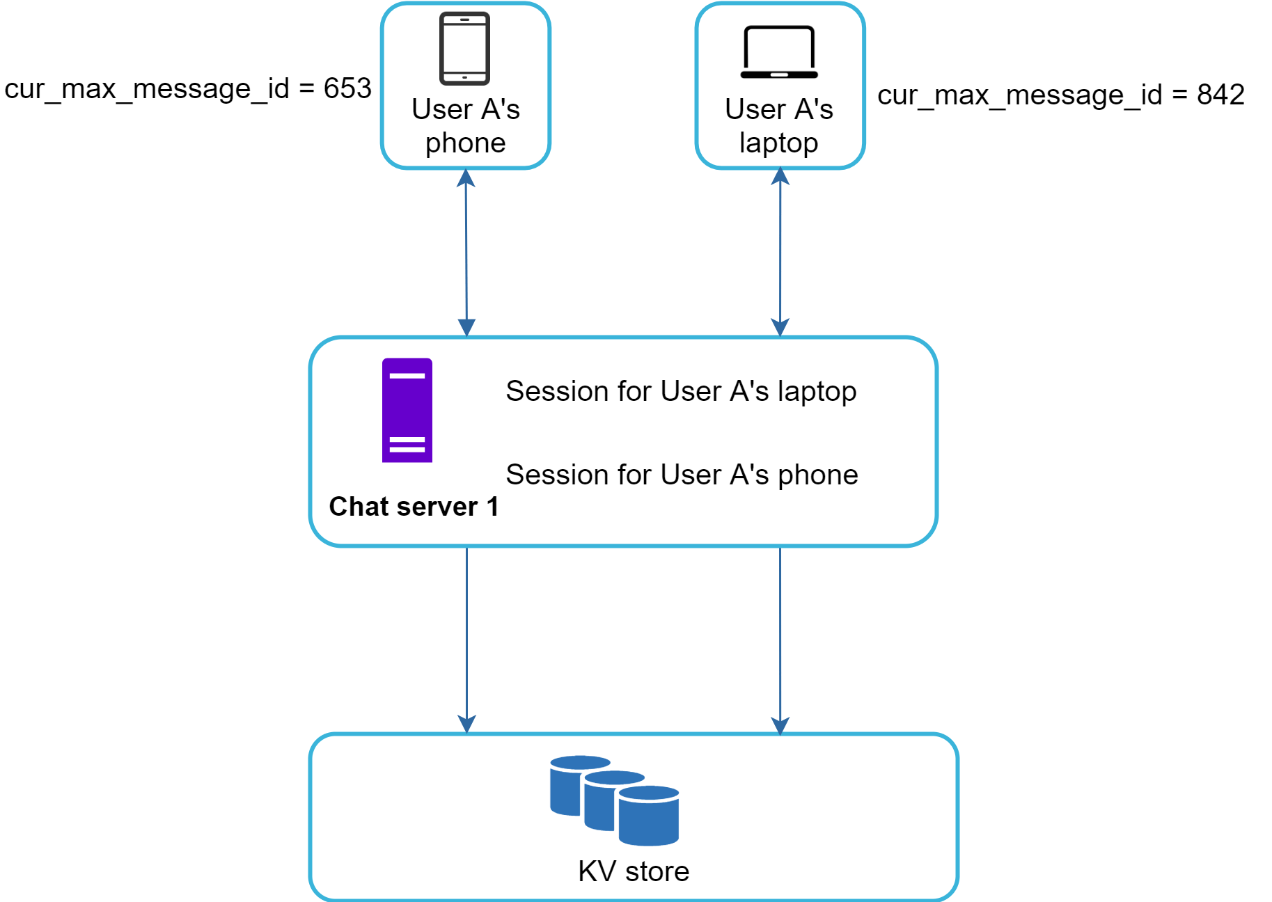
Small group chat flow
Figure 14 shows what happens when User A sends a message in a group chat (3 members: A, B, C). The message from User A is copied to each group member's message sync queue — one for User B and one for User C. Think of the message sync queue as an inbox for a recipient.
This design is good for small group chat because: - Simplifies message sync flow — each client only needs to check its own inbox. - Storing a copy in each recipient's inbox is not too expensive for small groups.
WeChat limits groups to 500 members [8]. For larger groups, storing a message copy for each member is not acceptable.
Figure 15 shows the recipient side: each recipient has an inbox (message sync queue) containing messages from different senders.
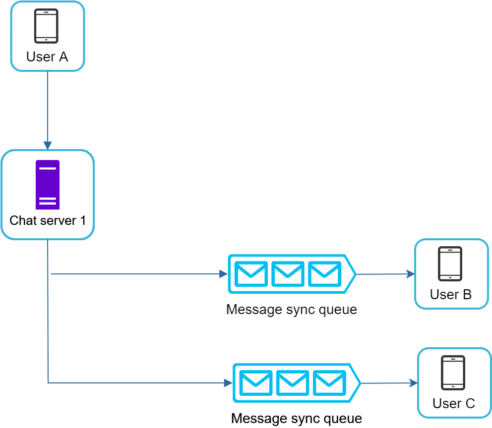
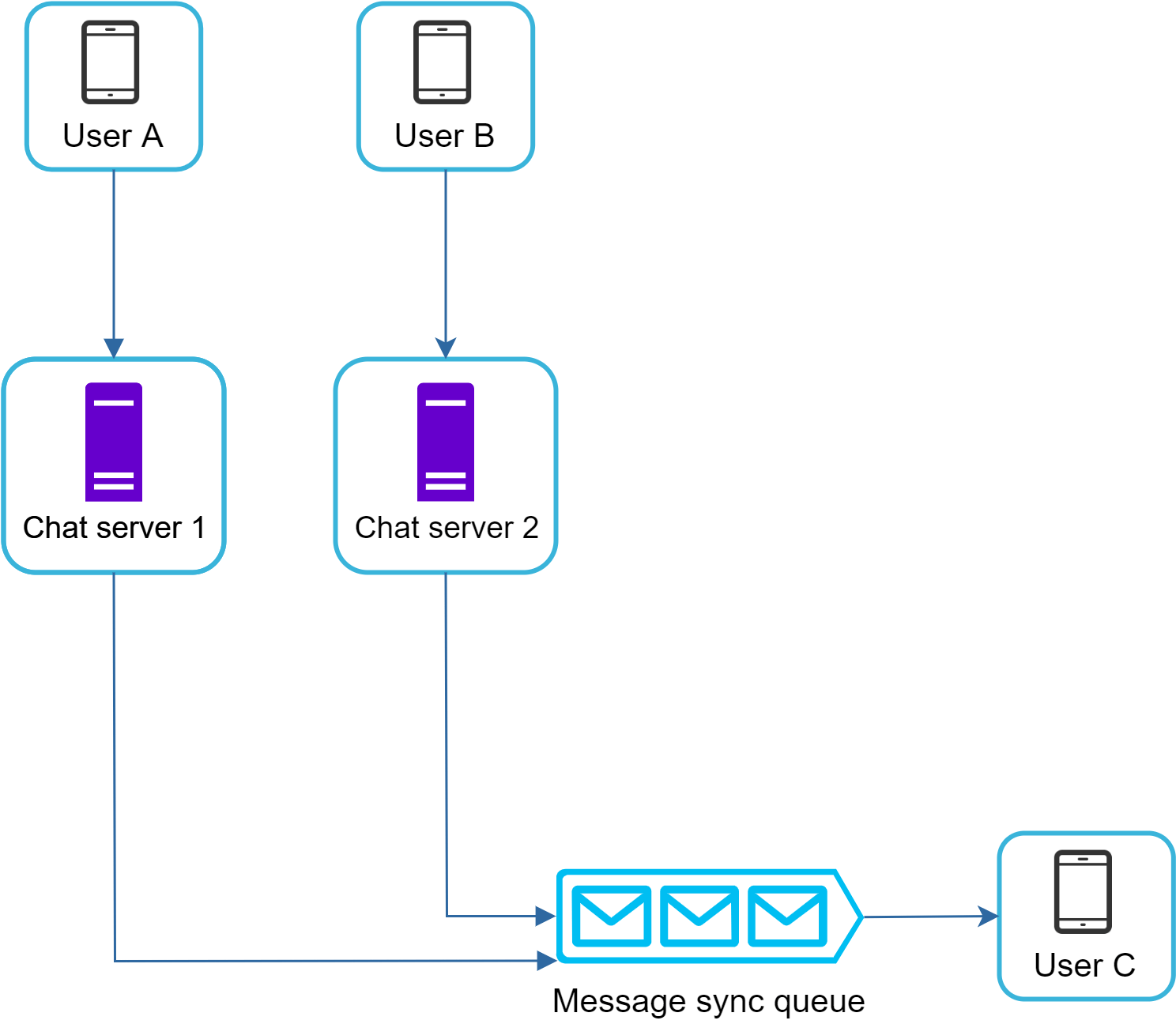
Online presence
Presence servers manage online status and communicate with clients through WebSocket.
**User login (Figure 16):** After WebSocket connection is built, User A's online status and `last_active_at` timestamp are saved in the KV store.
**User logout (Figure 17):** Online status is changed to offline in the KV store.
**User disconnection:** A naive approach (mark offline on disconnect, online on reconnect) causes poor UX because users frequently disconnect/reconnect briefly (e.g., going through a tunnel).
**Heartbeat mechanism (Figure 18):** Online clients send a heartbeat event to presence servers periodically. If presence servers receive a heartbeat within x seconds, the user is considered online. Otherwise, offline. Example: client sends heartbeat every 5 seconds; if no heartbeat for 30 seconds, status changes to offline.
**Online status fanout (Figure 19):** Presence servers use a publish-subscribe model. Each friend pair maintains a channel. When User A's status changes, it publishes to channels A-B, A-C, A-D. Those channels are subscribed by User B, C, D respectively.
For large groups (100,000 members), publishing a status change generates 100,000 events — too expensive. Solution: fetch online status only when a user enters a group or manually refreshes the friend list.
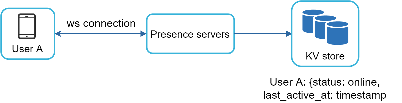
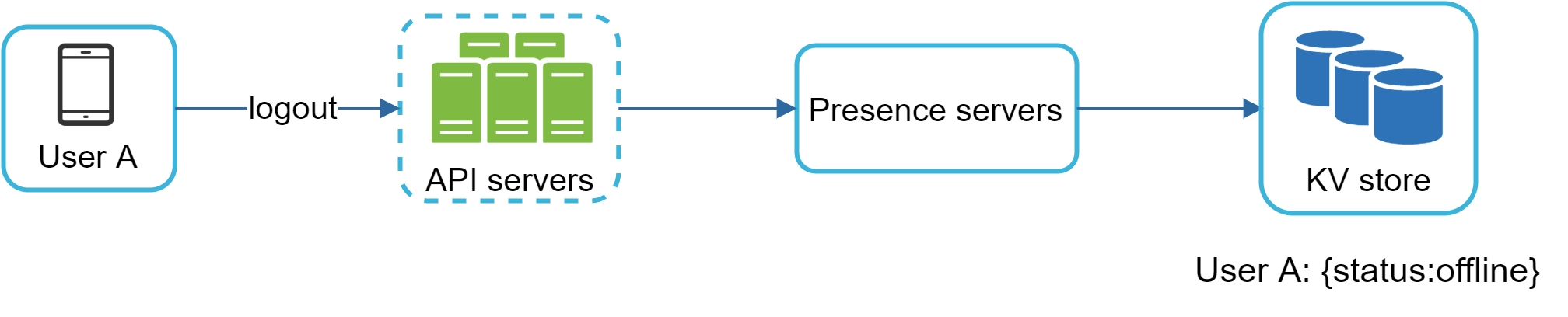

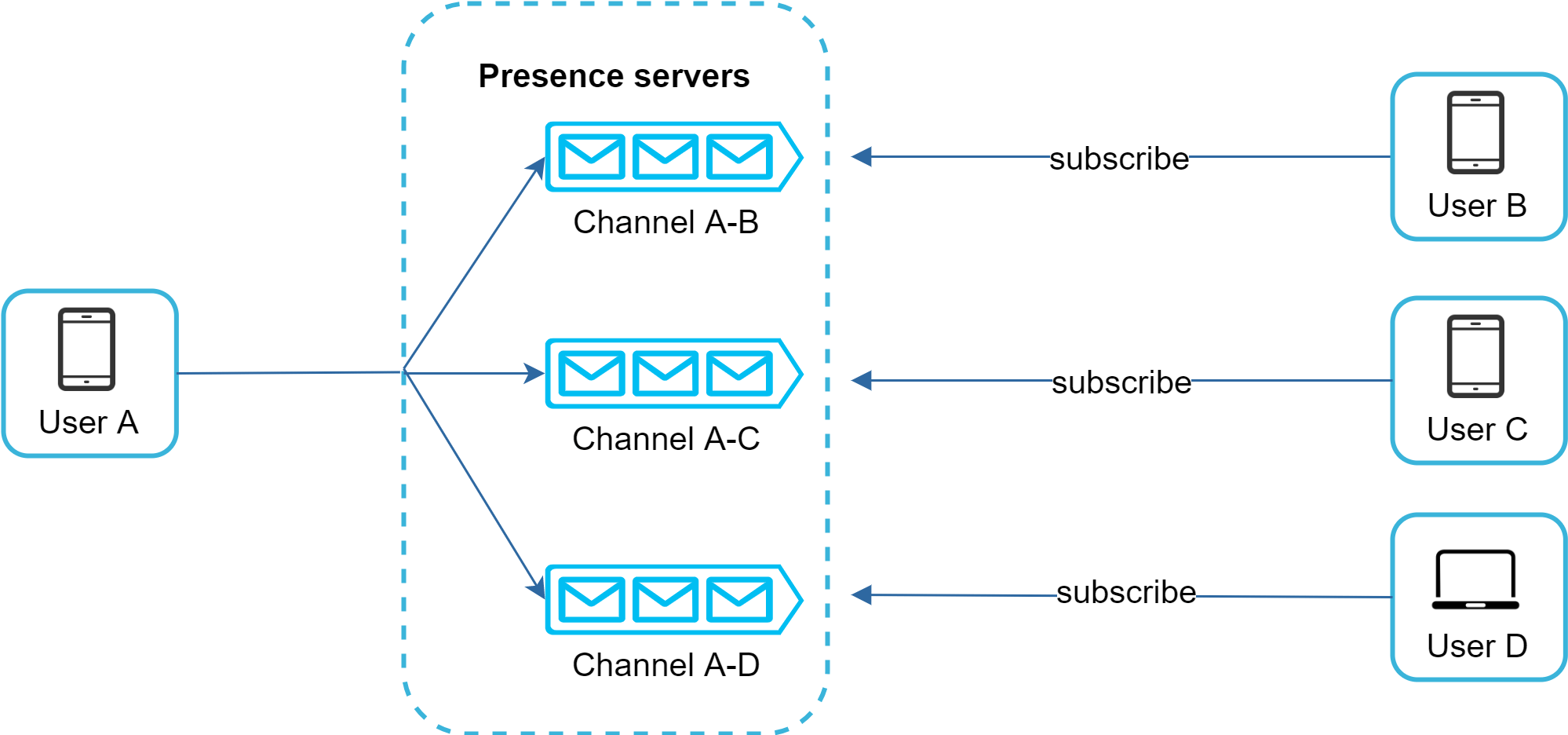
Step 4 - Wrap up
We presented a chat system supporting both 1-to-1 and small group chat. WebSocket is used for real-time communication. Components: chat servers, presence servers, push notification servers, key-value stores, API servers.
**Additional talking points:**
- **Media files:** Compression, cloud storage, and thumbnails for photos and videos. - **End-to-end encryption:** Only sender and recipient can read messages (like WhatsApp [9]). - **Client-side caching:** Reduces data transfer between client and server. - **Geographically distributed network:** Slack's approach to cache users' data for better load time [10]. - **Error handling:** - Chat server error: Service discovery (Zookeeper) provides a new chat server for reconnection. - Message resend mechanism: Retry and queueing for failed message delivery.
Design A Search Autocomplete System
When searching on Google or shopping at Amazon, as you type in the search box, one or more matches for the search term are presented to you. This feature is referred to as autocomplete, typeahead, search-as-you-type, or incremental search. This leads us to the interview question: design a search autocomplete system, also called "design top k" or "design top k most searched queries".
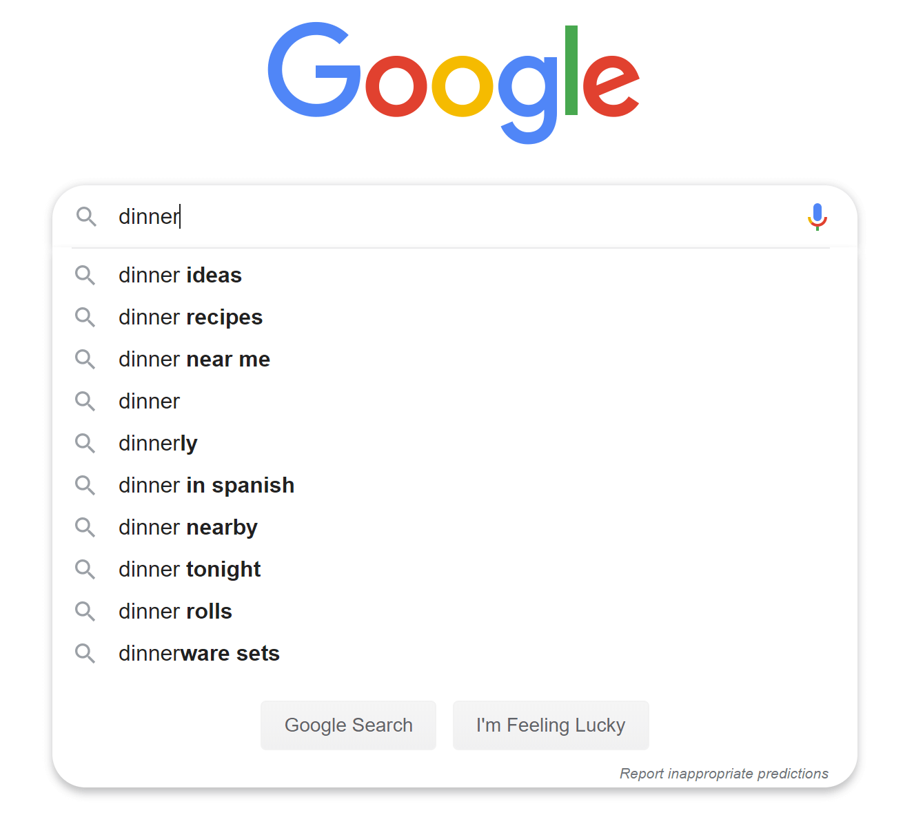
Step 1 - Understand the problem and establish design scope
**Requirements:**
- Matching only supported at the beginning of a search query. - Return 5 autocomplete suggestions. - Suggestions determined by popularity (historical query frequency). - No spell check or autocorrect. - English queries only (lowercase alphabetic characters). - 10 million DAU.
**Key non-functional requirements:** - Fast response time: must return results within 100 milliseconds [1]. - Relevant: suggestions relevant to the search term. - Sorted: results sorted by popularity or ranking models. - Scalable and highly available.
**Back of the envelope estimation:** - 10M DAU × 10 searches/day × 20 characters/query = ~24,000 QPS (peak: ~48,000) - 20% new queries daily: 10M × 10 × 20 bytes × 20% = **0.4 GB new data/day**
Step 2 - Propose high-level design and get buy-in
The system breaks down into two components:
- **Data gathering service:** Gathers user input queries and aggregates them in real-time (starting point; optimized in deep dive). - **Query service:** Given a search query or prefix, returns the 5 most frequently searched terms.
Data gathering service
A simplified frequency table stores query strings and their frequencies. Figure 2 shows how the frequency table is updated as users enter queries "twitch", "twitter", "twitter", and "twillo" sequentially.

Query service
Given a frequency table with Query and Frequency fields, when a user types "tw", the top 5 searched queries are displayed (Figure 3).
**Sample frequency table (Table 1):**
| Query | Frequency | |-------|-----------| | twitter | 35 | | twitch | 29 | | twilight | 25 | | twin peak | 21 | | twitch prime | 18 | | twitter search | 14 | | twillo | 10 | | twin peak sf | 8 |
The SQL query to get top 5 is shown in Figure 4. This is acceptable when the data set is small; accessing the database becomes a bottleneck for large data sets.
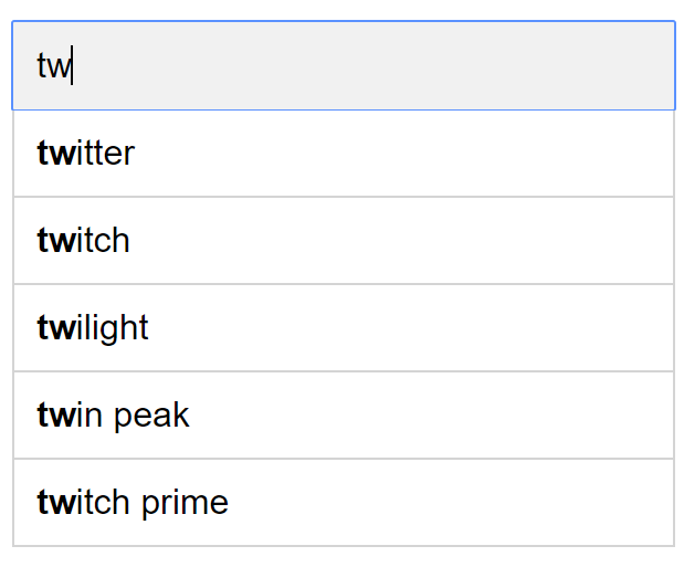
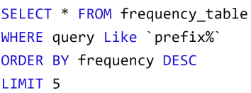
Step 3 - Design deep dive
Deep dive topics: trie data structure, data gathering service, query service, scale the storage, trie operations.
Trie data structure
Fetching top 5 queries from a relational database is inefficient. The **trie (prefix tree)** data structure overcomes this.
**Basic trie:** A tree-like data structure that compactly stores strings. The root represents an empty string. Each node stores a character and has 26 children (one per possible character). Each tree node represents a single word or prefix.
Figure 5 shows a trie with queries "tree", "try", "true", "toy", "wish", "win".
To support sorting by frequency, frequency info is included in nodes (Figure 6).
**Algorithm to get top k most searched queries:**
Define: p = prefix length, n = total nodes in trie, c = children of a node.
1. Find the prefix. Time: O(p) 2. Traverse subtree from prefix node to get all valid children. Time: O(c) 3. Sort children and get top k. Time: O(c log c)
Figure 7 shows the algorithm for k=2 and prefix "tr": - Step 1: Find prefix node "tr". - Step 2: Traverse subtree: [tree: 10], [true: 35], [try: 29]. - Step 3: Sort and get top 2: [true: 35] and [try: 29].
Total time complexity: O(p) + O(c) + O(c log c) — too slow for worst case.
**Two optimizations:**
1. **Limit max prefix length:** Users rarely type long queries, so limit p to ~50. Reduces "Find prefix" from O(p) to O(1).
2. **Cache top search queries at each node (Figure 8):** Store top k queries at each node. For example, node "be" stores [best: 35, bet: 29, bee: 20, be: 15, beer: 10]. With both optimizations, the algorithm takes O(1) total.


Data gathering service
Updating the trie on every query is not practical (billions of queries/day; top suggestions don't change much). Figure 9 shows the redesigned data gathering service.
**Components:** - **Analytics Logs:** Append-only raw data about search queries. - **Aggregators:** Aggregate raw data for processing. Trie rebuilt weekly for most use cases. - **Aggregated Data:** Weekly aggregated query + frequency table. - **Workers:** Async servers that build the trie and store it in Trie DB. - **Trie Cache:** Distributed cache keeping trie in memory for fast reads (weekly snapshot of DB). - **Trie DB:** Persistent storage. Two options: 1. Document store (MongoDB) — serialize trie snapshot weekly. 2. Key-value store — map every trie prefix to a key, trie node data to a value (Figure 10).


Query service
Figure 11 shows the improved query service design:
1. Search query sent to load balancer. 2. Load balancer routes to API servers. 3. API servers get trie data from Trie Cache and construct autocomplete suggestions. 4. Cache miss → replenish data from Trie DB back to cache.
**Optimizations:** - **AJAX request:** Browser sends async requests; doesn't refresh the whole page. - **Browser caching (Figure 12):** Autocomplete suggestions cached in browser (e.g., Google caches for 1 hour via `cache-control: private, max-age=3600`). - **Data sampling:** Only 1 out of N requests logged to reduce storage and processing overhead.
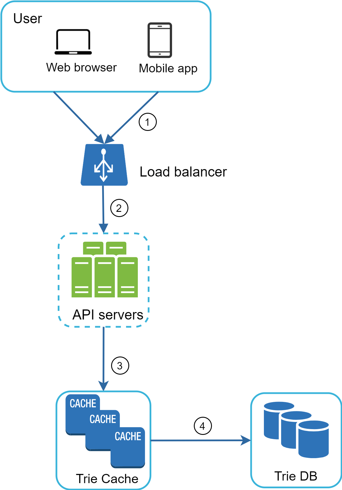
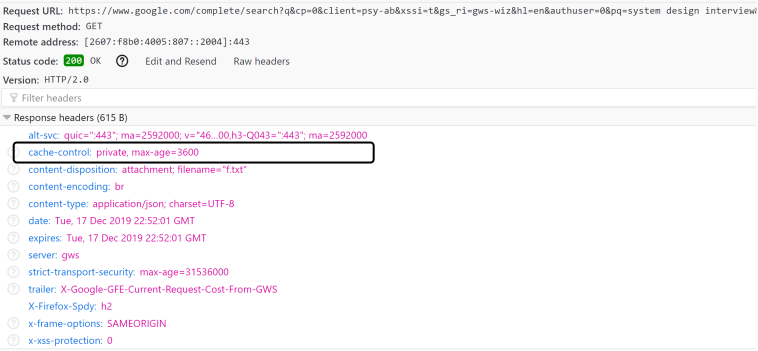
Trie operations
**Create:** Trie is built by workers using aggregated data from Analytics Log/DB.
**Update — two options:** 1. Replace the entire trie weekly with a freshly built one. 2. Update individual nodes directly (slow; when updating a node, all ancestors up to the root must be updated). Figure 13 shows updating "beer" from 10 to 30 — all ancestors are updated.
**Delete:** Remove hateful, violent, or dangerous autocomplete suggestions. A filter layer is added in front of the Trie Cache (Figure 14) to filter unwanted suggestions. Physical removal from the DB is done asynchronously for the next update cycle.

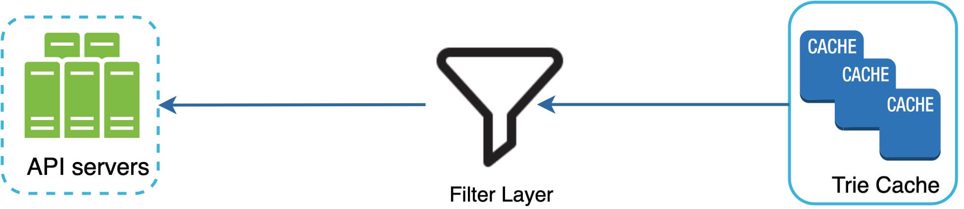
Scale the storage
When the trie grows too large for one server, shard based on the first character (up to 26 servers). For more servers, shard on second or third character level.
Naive first-character sharding creates uneven distribution (many more words starting with 'c' than 'x'). To mitigate imbalance, analyze historical data distribution and apply smarter sharding via a shard map manager (Figure 15). The shard map maintains a lookup DB identifying where rows should be stored.

Step 4 - Wrap up
**Additional talking points:**
- **Multi-language support:** Store Unicode characters in trie nodes. - **Country-specific top queries:** Build different tries per country; store in CDNs for faster response. - **Trending (real-time) search queries:** More complex — requires: - Reduced working data set by sharding. - Changed ranking model with more weight to recent queries. - Stream processing systems: Apache Hadoop MapReduce [6], Spark Streaming [7], Apache Storm [8], Apache Kafka [9].
Design YouTube
In this chapter, you are asked to design YouTube. The solution can be applied to other video sharing platforms such as Netflix and Hulu.
**YouTube statistics (2020):** - 2 billion monthly active users. - 5 billion videos watched per day. - 73% of US adults use YouTube. - 50 million creators. - $15.1 billion ad revenue in 2019 (up 36% from 2018). - Responsible for 37% of all mobile internet traffic. - Available in 80 languages.
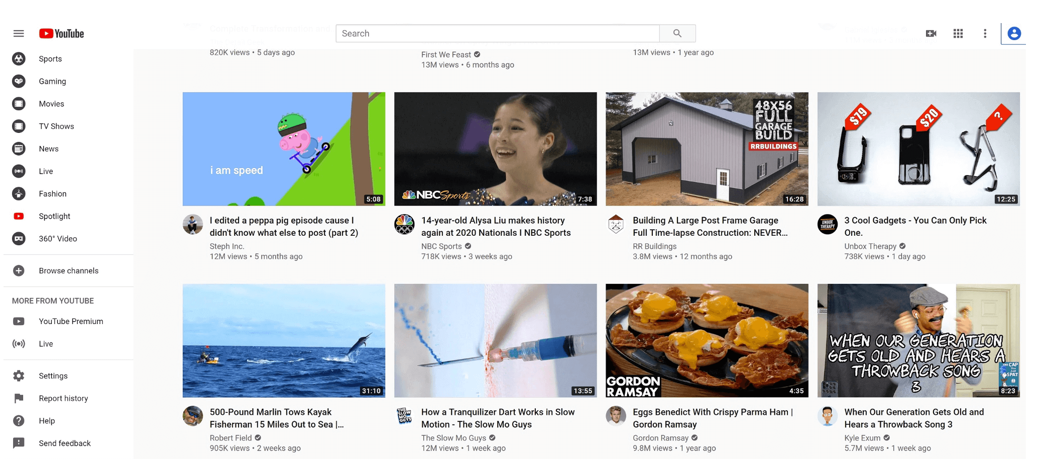
Step 1 - Understand the problem and establish design scope
**Requirements:** - Features: ability to upload a video and watch a video. - Clients: mobile apps, web browsers, smart TV. - 5 million DAU. - Average 30 minutes/day on product. - International users supported. - Most video resolutions and formats accepted. - Encryption required. - Maximum video size: 1 GB. - Can leverage existing cloud infrastructure (Amazon, Google, Microsoft).
**Focus features:** - Fast video upload - Smooth video streaming - Ability to change video quality - Low infrastructure cost - High availability, scalability, and reliability
**Back of the envelope estimation:** - Total daily storage: 5M × 10% upload × 300 MB = **150 TB/day** - CDN cost (CloudFront): 5M × 5 videos × 0.3 GB × $0.02/GB = **$150,000/day**
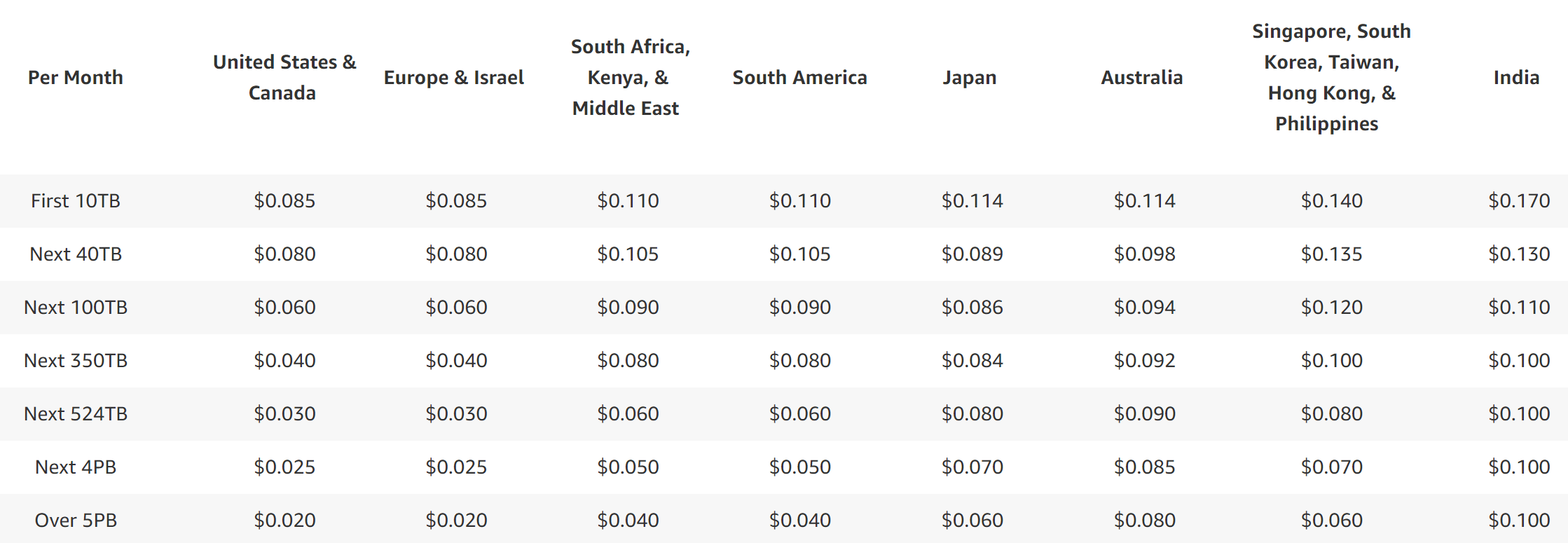
Step 2 - Propose high-level design and get buy-in
We leverage existing cloud services (CDN and blob storage) rather than building everything from scratch — building scalable blob storage or CDN is extremely complex (Netflix uses AWS [4], Facebook uses Akamai CDN [5]).
The system has three components (Figure 3): - **Client:** Computer, mobile phone, smartTV. - **CDN:** Videos stored in CDN; streamed from CDN when playing. - **API servers:** Everything except video streaming (feed recommendation, upload URL generation, metadata DB/cache, user signup, etc.).
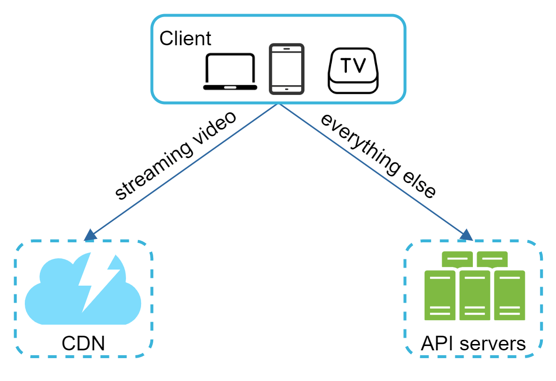
Video uploading flow
Figure 4 shows the high-level video uploading flow with these components: - **User, Load balancer, API servers** - **Metadata DB:** Sharded and replicated for performance and high availability. - **Metadata cache:** Caches video metadata and user objects. - **Original storage:** Blob storage for original videos. - **Transcoding servers:** Convert video to other formats (MPEG, HLS, etc.) for different devices/bandwidth. - **Transcoded storage:** Blob storage for transcoded videos. - **CDN:** Videos cached in CDN; streamed from here. - **Completion queue:** Message queue for video transcoding completion events. - **Completion handler:** Workers that pull events and update metadata cache and database.
The flow runs two parallel processes:
**Flow a — Upload the actual video (Figure 5):** 1. Video uploaded to original storage. 2. Transcoding servers fetch and transcode the video. 3. In parallel: - 3a. Transcoded videos → transcoded storage → CDN. - 3b. Transcoding completion events → completion queue → completion handler → metadata DB/cache. 4. API servers notify client that video is ready for streaming.
**Flow b — Update video metadata (Figure 6):** While uploading, client sends parallel request to update metadata (file name, size, format). API servers update metadata cache and database.
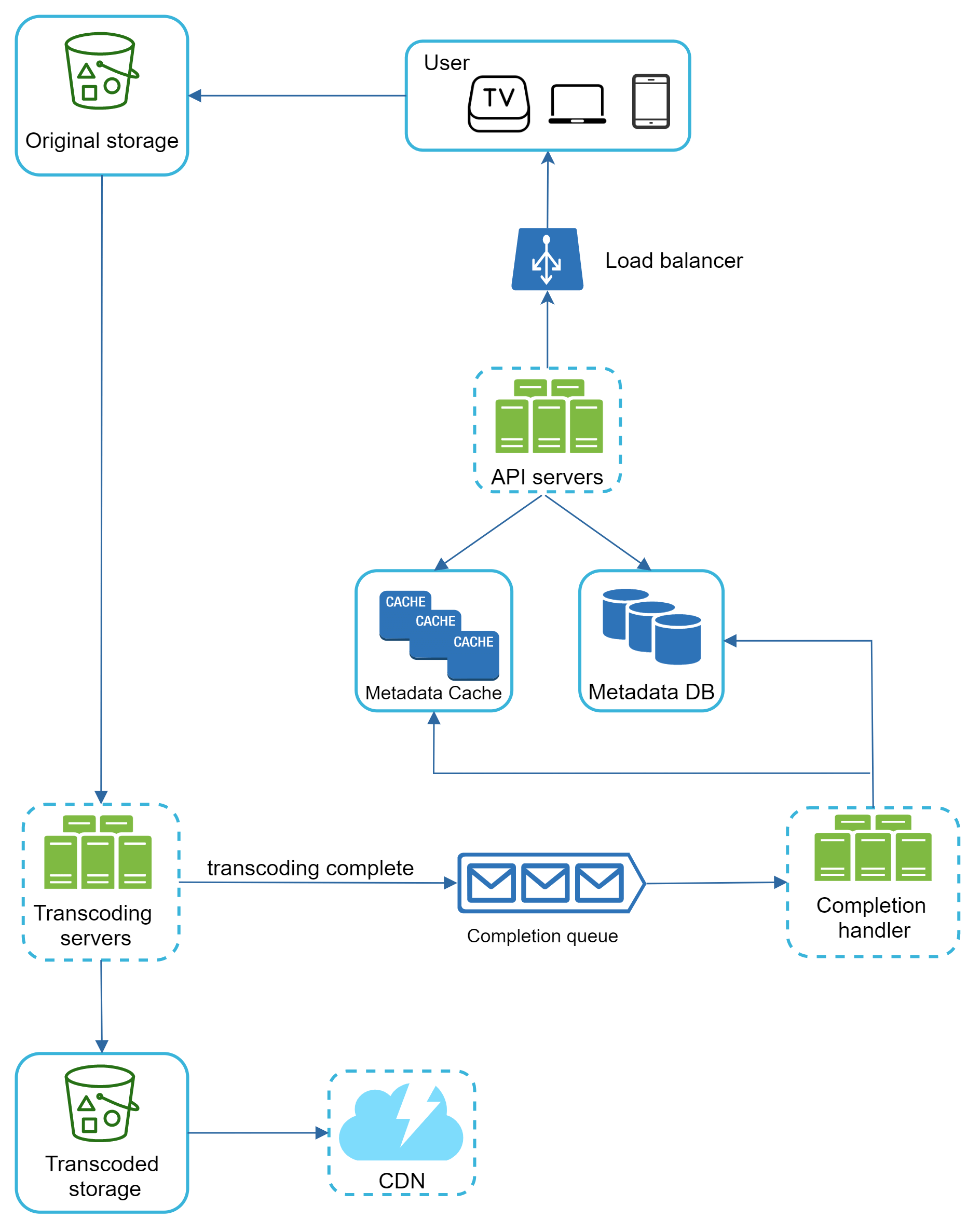
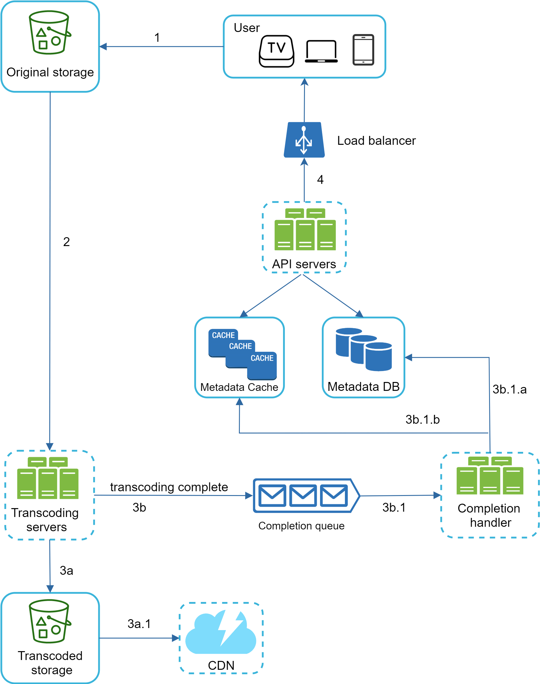
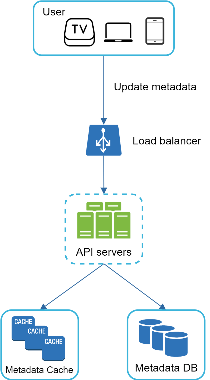
Video streaming flow
Streaming means continuously receiving small chunks — users can watch immediately without downloading the entire video.
**Popular streaming protocols:** - MPEG-DASH (Moving Picture Experts Group — Dynamic Adaptive Streaming over HTTP) - Apple HLS (HTTP Live Streaming) - Microsoft Smooth Streaming - Adobe HTTP Dynamic Streaming (HDS)
Videos are streamed from the CDN directly; the edge server closest to the user delivers the video with minimal latency (Figure 7).
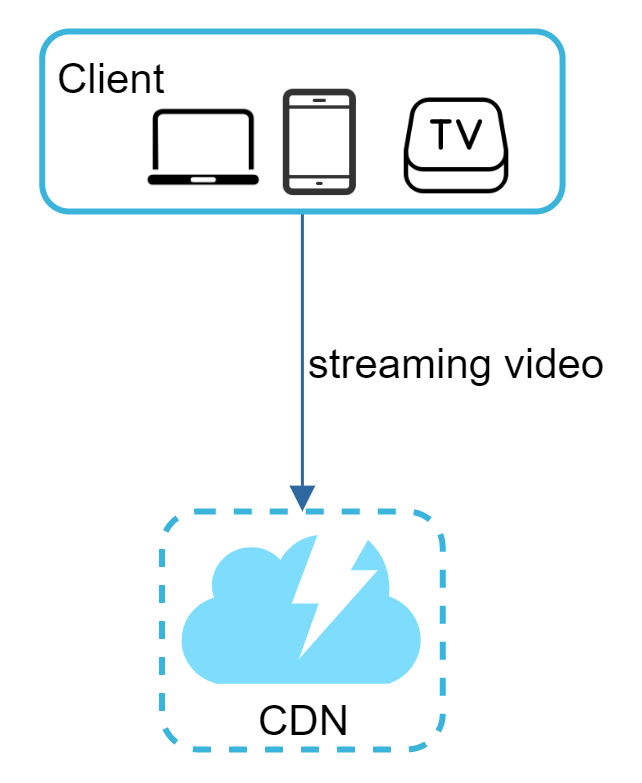
Step 3 - Design deep dive
We refine both flows with optimizations and error handling mechanisms.
Video transcoding
**Why transcoding is important:** - Raw video is huge (60fps HD hour-long video = hundreds of GB). - Many devices/browsers only support certain video formats. - Deliver higher resolution for high-bandwidth users, lower for slow connections. - Network conditions change, especially on mobile — adaptive quality is essential.
**Encoding formats have two parts:** - **Container:** Basket for video, audio, metadata (`.avi`, `.mov`, `.mp4`). - **Codecs:** Compression/decompression algorithms (H.264, VP9, HEVC).
Directed acyclic graph (DAG) model
Transcoding is expensive and different creators have different requirements (watermarks, thumbnails, HD). We adopt a DAG model inspired by Facebook's streaming video engine [8] to support different video processing pipelines with high parallelism.
Figure 8 shows a DAG for video transcoding. The original video is split into video, audio, and metadata. Tasks that can be applied: - **Inspection:** Ensure video has good quality and is not malformed. - **Video encodings:** Convert to different resolutions, codecs, bitrates (Figure 9). - **Thumbnail:** Uploaded by user or auto-generated. - **Watermark:** Image overlay with identifying information.


Video transcoding architecture
Figure 10 shows the transcoding architecture with six main components:
**Preprocessor (Figure 11):** Four responsibilities: 1. Video splitting into GOP (Group of Pictures) aligned chunks — independently playable units, usually a few seconds. 2. Handle old devices that don't support client-side splitting. 3. DAG generation from configuration files (Figure 12, Figure 13). 4. Cache segmented videos (GOPs + metadata) in temporary storage for retry on failure.
**DAG scheduler (Figure 14):** Splits a DAG graph into task stages and puts them in the resource manager's task queue. Figure 15 shows stages: Stage 1 (video/audio/metadata), Stage 2 (video encoding + thumbnail, audio encoding).
**Resource manager (Figure 16):** Manages resource allocation efficiency with 3 queues and a task scheduler (Figure 17): - **Task queue:** Priority queue of tasks to execute. - **Worker queue:** Priority queue of worker utilization info. - **Running queue:** Currently running tasks and workers. - **Task scheduler:** Picks optimal task/worker, instructs worker to run the job, manages the running queue.
**Task workers (Figure 18):** Run tasks defined in the DAG. Different workers run different tasks (Figure 19).
**Temporary storage (Figure 20):** Multiple storage systems — metadata cached in memory, video/audio in blob storage. Freed once video processing completes.
**Encoded video (Figure 21):** Final output (e.g., `funny_720p.mp4`).


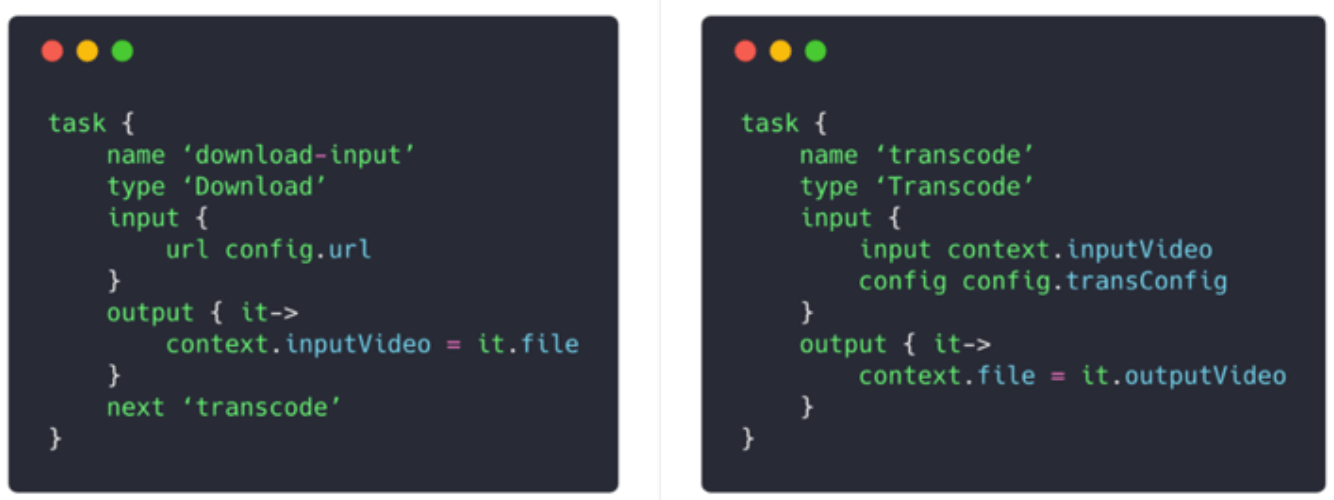


System optimizations
**Speed — parallelize video uploading (Figure 22):** Split video into GOP-aligned chunks. Enables fast resumable uploads on failure. Client handles splitting (Figure 23).
**Speed — upload centers close to users (Figure 24):** Multiple upload centers globally (North America, Asia, etc.) using CDN as upload centers.
**Speed — parallelism everywhere (Figure 25, 26):** Sequential flow (Figure 25) makes parallelism difficult. After introducing message queues (Figure 26), the encoding module doesn't wait for the download module — events in the queue can be processed independently.
**Safety — pre-signed upload URL (Figure 27):** Flow: 1. Client requests pre-signed URL from API servers. 2. API servers return pre-signed URL. 3. Client uploads video using the pre-signed URL. (AWS calls it pre-signed URL; Azure calls it "Shared Access Signature" [10])
**Safety — video protection options:** - Digital rights management (DRM): Apple FairPlay, Google Widevine, Microsoft PlayReady. - AES encryption with authorization policy. - Visual watermarking.
**Cost savings (Figure 28):** YouTube follows long-tail distribution [11][12] — few popular videos get most views. 1. Serve only the most popular videos from CDN; others from high-capacity storage servers. 2. Less popular content encoded on-demand (fewer versions stored). 3. Region-specific popular videos not distributed globally. 4. Build own CDN like Netflix and partner with ISPs.

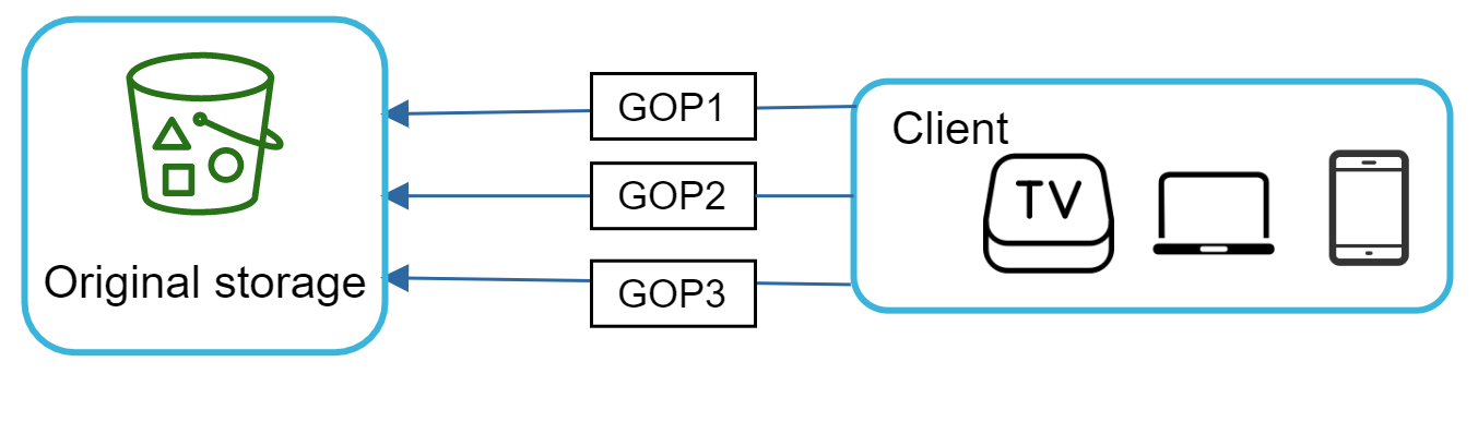


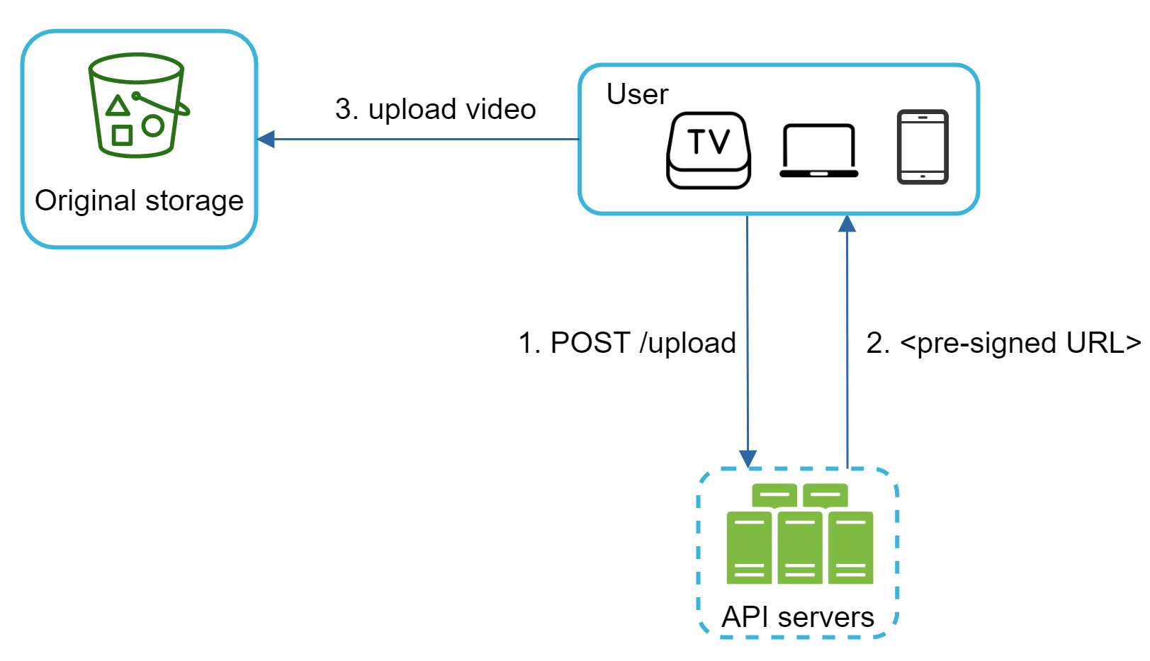
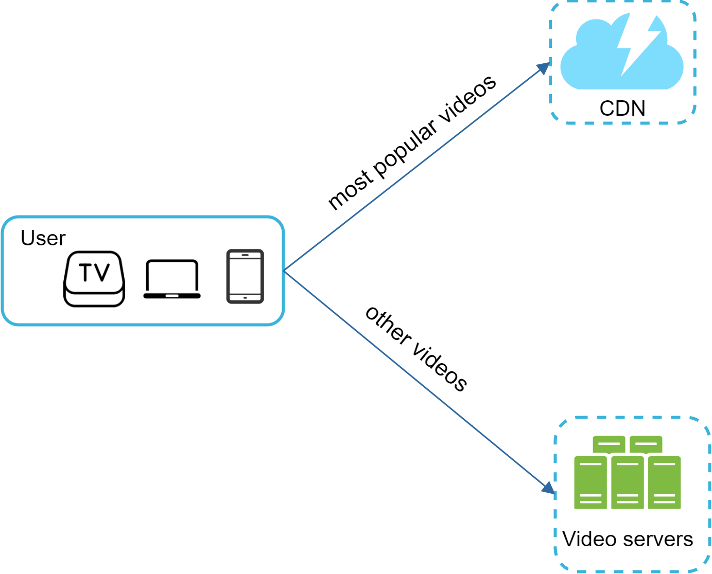
Error handling
**Recoverable errors** (e.g., segment fails to transcode): retry a few times, then return error code. **Non-recoverable errors** (e.g., malformed video): stop tasks and return error code.
**Error playbook by component:** - Upload error: retry. - Split video error: server handles splitting if old client can't. - Transcoding error: retry. - Preprocessor error: regenerate DAG. - DAG scheduler error: reschedule task. - Resource manager queue down: use a replica. - Task worker down: retry on new worker. - API server down: route to another stateless API server. - Metadata cache down: read from replicas; bring up new cache server. - Metadata DB master down: promote a slave to master. - Metadata DB slave down: use another slave; bring up a replacement.
Step 4 - Wrap up
**Additional talking points:** - **Scale API tier:** Stateless API servers scale horizontally. - **Scale database:** Replication and sharding. - **Live streaming:** Higher latency requirements, different streaming protocol, less parallelism (real-time small chunks), different error handling. - **Video takedowns:** Remove copyright violations, pornography, illegal content — discovered during upload or through user flagging.
Design Google Drive
In this chapter, you are asked to design Google Drive — a file storage and synchronization service that helps you store documents, photos, videos, and other files in the cloud, accessible from any computer, smartphone, and tablet.
Step 1 - Understand the problem and establish design scope
**Features in scope:** - Add files (drag and drop). - Download files. - Sync files across multiple devices. - See file revisions. - Share files with friends, family, coworkers. - Send notifications when a file is edited, deleted, or shared.
**Out of scope:** Google Docs editing and collaboration.
**Requirements:** - Any file type; files must be encrypted. - Max file size: 10 GB. - 10M DAU.
**Non-functional requirements:** - Reliability: data loss is unacceptable. - Fast sync speed. - Minimal bandwidth usage. - Scalable and highly available.
**Back of the envelope estimation:** - 50M users × 10 GB free = **500 PB total storage** - Upload QPS: 10M × 2 uploads / 86400 ≈ **240 QPS** (peak: 480)
Step 2 - Propose high-level design and get buy-in
Start with a single server setup, then scale up: - Web server to upload/download files. - MySQL database for metadata (user data, login, files). - `drive/` directory as root storage (1 TB).
Under `drive/`, a list of directories (namespaces) — each namespace contains all uploaded files for a user. Files uniquely identified by joining namespace and relative path.
Figure 3 shows the `drive/` directory structure.

APIs
Three primary APIs:
**1. Upload a file:** - Simple upload: small files. - Resumable upload: large files or unreliable networks. ``` POST https://api.example.com/files/upload?uploadType=resumable Params: uploadType=resumable, data: local file ``` Resumable upload steps: send initial request → retrieve resumable URL → upload data and monitor → resume if disturbed.
**2. Download a file:** ``` GET https://api.example.com/files/download Params: path: download file path ```
**3. Get file revisions:** ``` GET https://api.example.com/files/list_revisions Params: path, limit ```
All APIs require user authentication and use HTTPS/SSL.
Move away from single server
As more files are uploaded, storage fills up (Figure 4). Solution: shard data across multiple storage servers (Figure 5 — sharding by user_id).
To guard against data loss, use Amazon S3 — supports same-region and cross-region replication (Figure 6). Data replicated in multiple regions ensures availability and durability.
Further improvements: - **Load balancer:** Distribute traffic; redistribute when a web server goes down. - **More web servers:** Easily scale after adding load balancer. - **Metadata database:** Move out of single server; set up replication and sharding. - **File storage:** S3 with replication in two geographic regions.
Figure 7 shows the updated design with decoupled web servers, metadata database, and file storage.


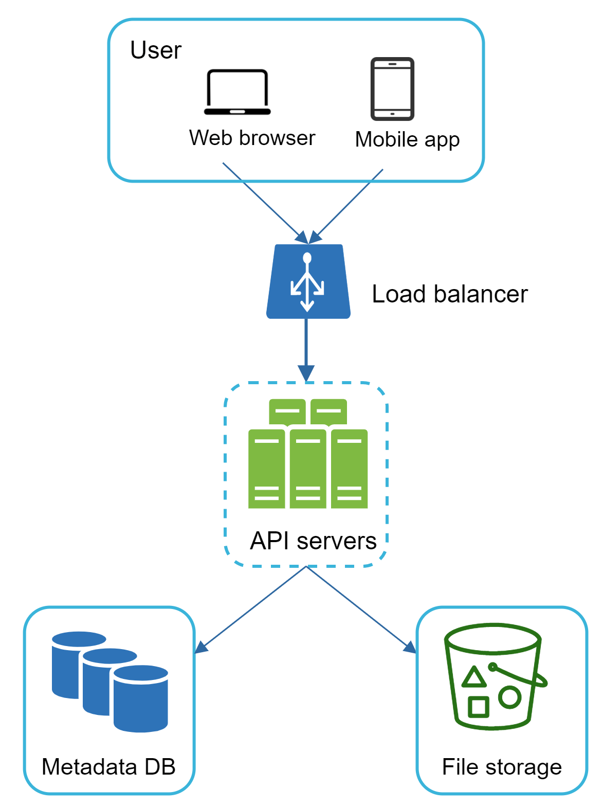
Sync conflicts
When two users modify the same file simultaneously, a conflict occurs. **Strategy: first version processed wins; later version receives a conflict (Figure 8).**
User 2 gets a sync conflict. The system presents both copies — user 2's local copy and the latest server version (Figure 9). User 2 can merge both files or override one version with the other.

High-level design
Figure 10 shows the proposed high-level design with components:
- **User:** Uses browser or mobile app. - **Block servers:** Upload blocks to cloud storage. Files split into blocks (max 4 MB each, like Dropbox [6]), each with a unique hash value. To reconstruct a file, blocks joined in order. - **Cloud storage:** File blocks stored in S3. - **Cold storage:** For inactive data (files not accessed for months/years). - **Load balancer:** Distributes requests among API servers. - **API servers:** User authentication, profile management, metadata updates. - **Metadata database:** Stores metadata of users, files, blocks, versions. - **Metadata cache:** Caches frequently accessed metadata. - **Notification service:** Publisher/subscriber system — notifies clients when a file is added/edited/removed elsewhere. - **Offline backup queue:** Stores pending changes for offline clients; synced when client comes online.
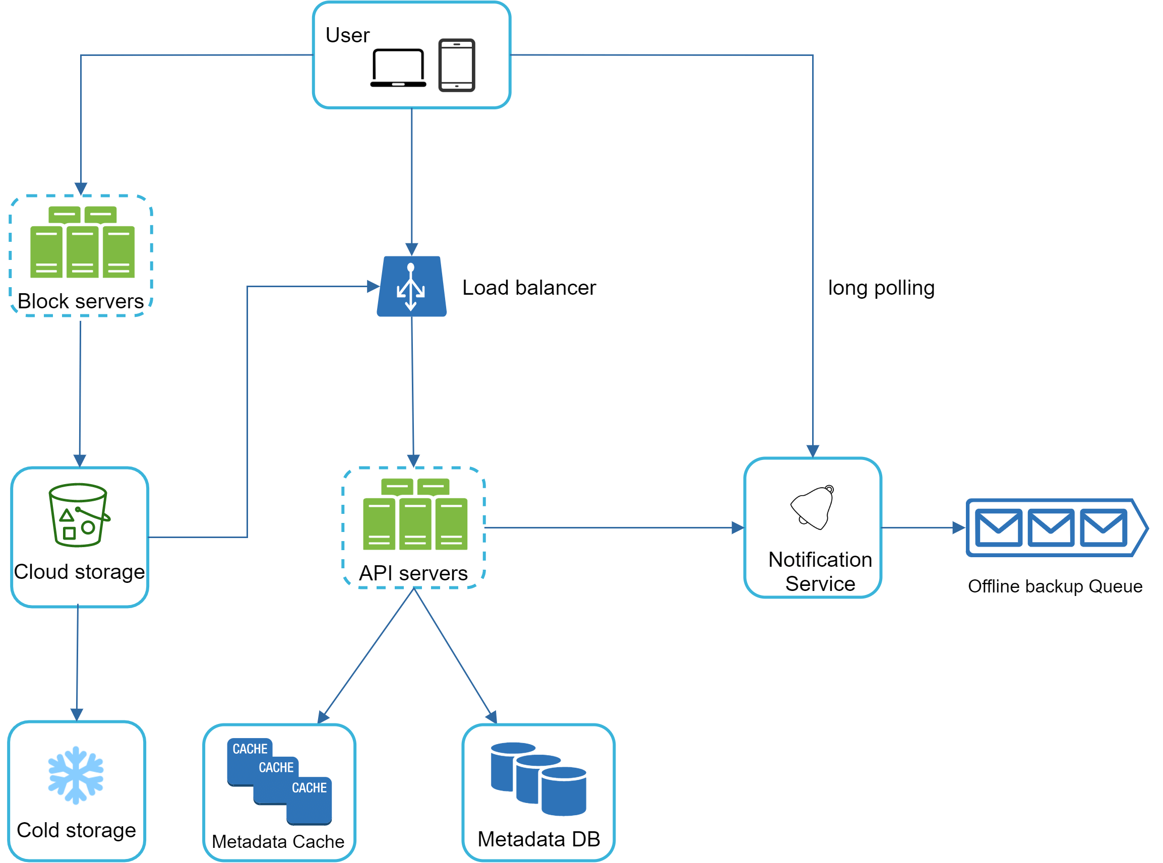
Step 3 - Design deep dive
Deep dive into: block servers, metadata database, upload flow, download flow, notification service, storage savings, failure handling.
Block servers
Two optimizations to minimize bandwidth:
1. **Delta sync:** Only modified blocks are synced instead of the whole file [7][8]. 2. **Compression:** Blocks compressed using algorithms depending on file type (gzip/bzip2 for text; different algorithms for images/videos).
Block server workflow for a new file (Figure 11): 1. File split into smaller blocks. 2. Each block compressed. 3. Each block encrypted before sending to cloud storage. 4. Blocks uploaded to cloud storage.
For delta sync (Figure 12): only modified blocks ("block 2" and "block 5") are uploaded to cloud storage.
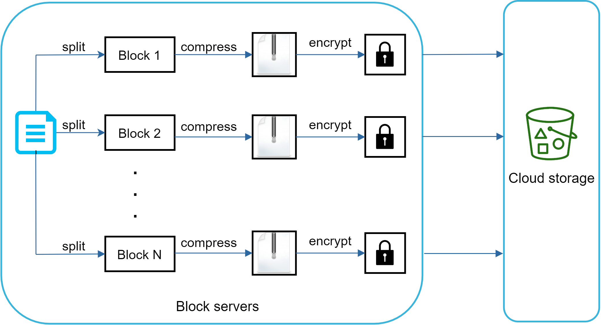

High consistency requirement
Strong consistency required — a file must not be shown differently by different clients simultaneously.
- Memory caches adopt eventual consistency by default — must ensure cache replicas and master are consistent. - Invalidate caches on database write. - We choose **relational databases** because ACID properties (Atomicity, Consistency, Isolation, Durability) are natively supported [9]. NoSQL databases don't support ACID by default.
Metadata database
Figure 13 shows the database schema (simplified):
- **User:** username, email, profile photo. - **Device:** device info, push_id for mobile push notifications. One user can have multiple devices. - **Namespace:** Root directory of a user. - **File:** Latest file information. - **File_version:** Version history. Existing rows are read-only to maintain integrity. - **Block:** Everything about a file block. Any version reconstructed by joining blocks in correct order.
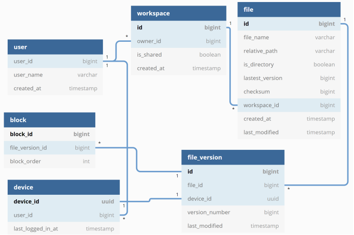
Upload flow
Figure 14 shows the sequence diagram for file upload. Two parallel requests from client 1:
**Add file metadata:** 1. Client 1 sends request to add metadata. 2. Store metadata in metadata DB with status "pending". 3. Notify notification service about new file. 4. Notification service notifies client 2.
**Upload file to cloud storage:** 2.1 Client 1 uploads content to block servers. 2.2 Block servers chunk, compress, encrypt, and upload blocks to cloud storage. 2.3 Cloud storage triggers upload completion callback to API servers. 2.4 File status changed to "uploaded" in metadata DB. 2.5-2.6 Notification service notifies client 2 that file is fully uploaded.

Download flow
Client knows a file changed via: - **Online:** Notification service informs client of changes. - **Offline:** Data saved to cache; pulled when client comes back online.
Figure 15 shows the download flow: 1. Notification service informs client 2 of a change. 2. Client 2 requests metadata from API servers. 3-4. API servers fetch metadata from metadata DB. 5. Client 2 receives metadata. 6. Client 2 requests blocks from block servers. 7-8. Block servers download blocks from cloud storage. 9. Client 2 downloads blocks and reconstructs the file.

Notification service
Options: **Long polling** (used by Dropbox [10]) vs **WebSocket**.
We choose **long polling** because: - Communication is one-directional (server → client for file changes). - Google Drive notifications are infrequent, not real-time streams like chat.
With long polling, each client establishes a long poll connection. On file change detection, client closes the connection, fetches latest changes from metadata server, then immediately re-opens the connection.
Save storage space
Three techniques to reduce storage costs:
1. **De-duplicate data blocks:** Two blocks are identical if they have the same hash value — eliminate redundant blocks at account level. 2. **Intelligent backup strategy:** - Set a limit on number of versions to store. - Keep only valuable versions (limit heavily modified files). 3. **Cold storage for infrequently accessed data:** Amazon S3 Glacier [11] is much cheaper than S3.
Failure Handling
- **Load balancer failure:** Secondary becomes active; heartbeat monitoring between load balancers. - **Block server failure:** Other servers pick up unfinished/pending jobs. - **Cloud storage failure:** S3 buckets replicated in different regions; fetch from another region. - **API server failure:** Stateless; traffic redirected by load balancer. - **Metadata cache failure:** Replicated; bring up new server to replace failed one. - **Metadata DB failure:** - Master down: promote a slave to master, bring up new slave. - Slave down: use another slave; bring up replacement. - **Notification service failure:** Over 1M connections per machine (per Dropbox 2012 [6]). On failure, all long poll connections lost; clients must reconnect slowly. - **Offline backup queue failure:** Queues replicated; consumers re-subscribe to backup queue.
Step 4 - Wrap up
We designed Google Drive with two flows: file metadata management and file sync. Notification service uses long polling to keep clients updated.
**Alternative design discussion:** - Upload files directly from client to cloud storage (bypassing block servers): faster, but requires chunking/compression/encryption logic on every client platform (error-prone, harder to maintain), and client-side encryption is a security risk. - **Presence service:** Move online/offline logic to a separate service for better modularity and reuse by other services.
Proximity Service
A proximity service is used to discover nearby places such as restaurants, hotels, theaters, museums, etc. It powers features like finding the best restaurants nearby on Yelp or finding k-nearest gas stations on Google Maps.
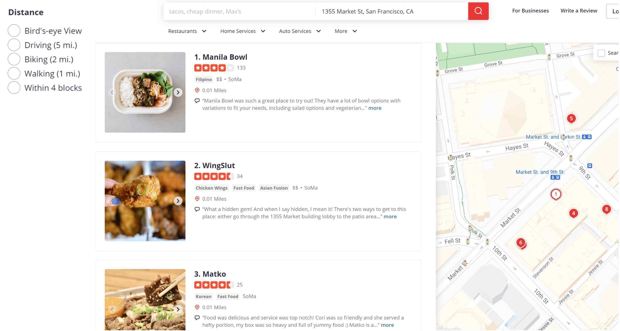
Step 1 - Understand the Problem and Establish Design Scope
**Functional requirements:** - Return all businesses based on a user's location (lat/long) and radius. - Business owners can add, delete, or update a business (not real-time; effective next day). - Customers can view detailed information about a business.
**Non-functional requirements:** - Low latency: users should see nearby businesses quickly. - Data privacy: comply with GDPR [4] and CCPA [5]. - High availability and scalability: handle spike traffic during peak hours in densely populated areas.
**Back of the envelope estimation:** - 100 million DAU, 200 million businesses. - Search QPS = 100M × 5 searches/day ÷ 10^5 seconds = **5,000 QPS**
Step 2 - Propose High-Level Design and Get Buy-In
API Design
**Search nearby businesses:** ``` GET /v1/search/nearby Params: latitude, longitude, radius (default 5000m) Response: { total: 10, businesses: [{business object}] } ```
**Business CRUD APIs:**
| API | Detail | |-----|--------| | GET /v1/businesses/{:id} | Return detailed information about a business | | POST /v1/businesses | Add a business | | PUT /v1/businesses/{:id} | Update details of a business | | DELETE /v1/businesses/{:id} | Delete a business |
Data model
Read-heavy system (search + view) with low write volume. Relational database (MySQL) is a good fit.
**Business table (Table 3):** Contains detailed business information with `business_id` as primary key.
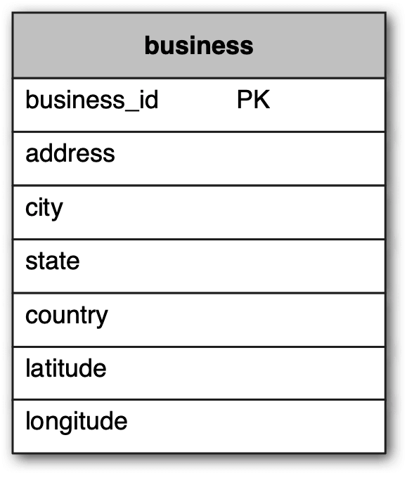
High-level design
Figure 2 shows the system with two parts: Location-Based Service (LBS) and business service.
- **Load balancer:** Distributes traffic; routes API calls based on URL paths. - **LBS (Location-Based Service):** Core component finding nearby businesses. Read-heavy, high QPS, stateless (easy to scale horizontally). - **Business service:** Handles write operations (add/update/delete) and detailed business info reads. - **Database cluster:** Primary-secondary setup. Primary handles writes; replicas handle reads. Slight replication delay is acceptable (business info not real-time).
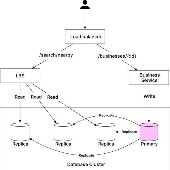
Algorithms to fetch nearby businesses
**Option 1: Two-dimensional search (Figure 3):** Draw a circle with predefined radius, find all businesses within it. SQL using latitude/longitude BETWEEN — requires full table scan. Even with indexes on both columns (Figure 4), intersecting two large datasets is inefficient.
**Geospatial indexing types (Figure 5):** - Hash: even grid, geohash, cartesian tiers. - Tree: quadtree, Google S2, RTree.
**Option 2: Evenly divided grid (Figure 6):** Divide world into equal grids. Problem: uneven business distribution — downtown NYC vs deserts/oceans.
**Option 3: Geohash** reduces 2D coordinates to 1D string. Recursively divides world into smaller grids with each additional bit.
Geohash division: - Divide planet into quadrants (Figure 7). - Each grid recursively divided into 4 (Figure 8). - Uses base32 representation.
Geohash length to grid size (Table 4): length 4 = 39.1×19.5km, length 5 = 4.9×4.9km, length 6 = 1.2km×609m.
Radius to geohash length (Table 5): 0.5km→6, 1km→5, 2km→5, 5km→4, 20km→4.
**Boundary issues:** - Issue 1 (Figure 9, 10): Two close locations can have NO shared prefix (e.g., opposite sides of equator). Simple prefix query fails. - Issue 2 (Figure 11): Two positions can have long shared prefix but belong to different geohashes. - Solution: fetch businesses from current grid AND all 8 neighbors.
**Not enough businesses (Figure 12):** Remove last digit of geohash to expand to larger grid; repeat until enough results.
**Option 4: Quadtree (Figure 13):** Recursively subdivide 2D space into 4 quadrants until grid has ≤100 businesses. In-memory structure built at server start-up.
Building process (Figure 14): - Total memory: ~1.71 GB for 200M businesses. - Build time: a few minutes at startup; use rolling deployment to avoid service disruption.
Real-world quadtree example near Denver (Figure 15): smaller grids for dense areas, larger for sparse.
**Option 5: Google S2 (Figure 16):** Maps sphere to 1D index via Hilbert curve. Two points close on Hilbert curve are close in 1D. Supports geofencing (Figure 17) — define perimeters and send notifications to users outside.
**Recommendation:**
| Geo Index | Companies | |-----------|----------| | Geohash | Bing map, Redis, MongoDB, Lyft | | Quadtree | Yext | | Both | Elasticsearch | | S2 | Google Maps, Tinder |
Choose geohash or quadtree for interviews (S2 too complex to explain).
**Geohash vs Quadtree:** - Geohash: easy to use/implement; supports radius search; fixed grid size; easy index updates (Figure 18). - Quadtree: supports k-nearest search; dynamically adjusts grid size based on density; more complex to implement and update (O(log n) traversal, Figure 19).
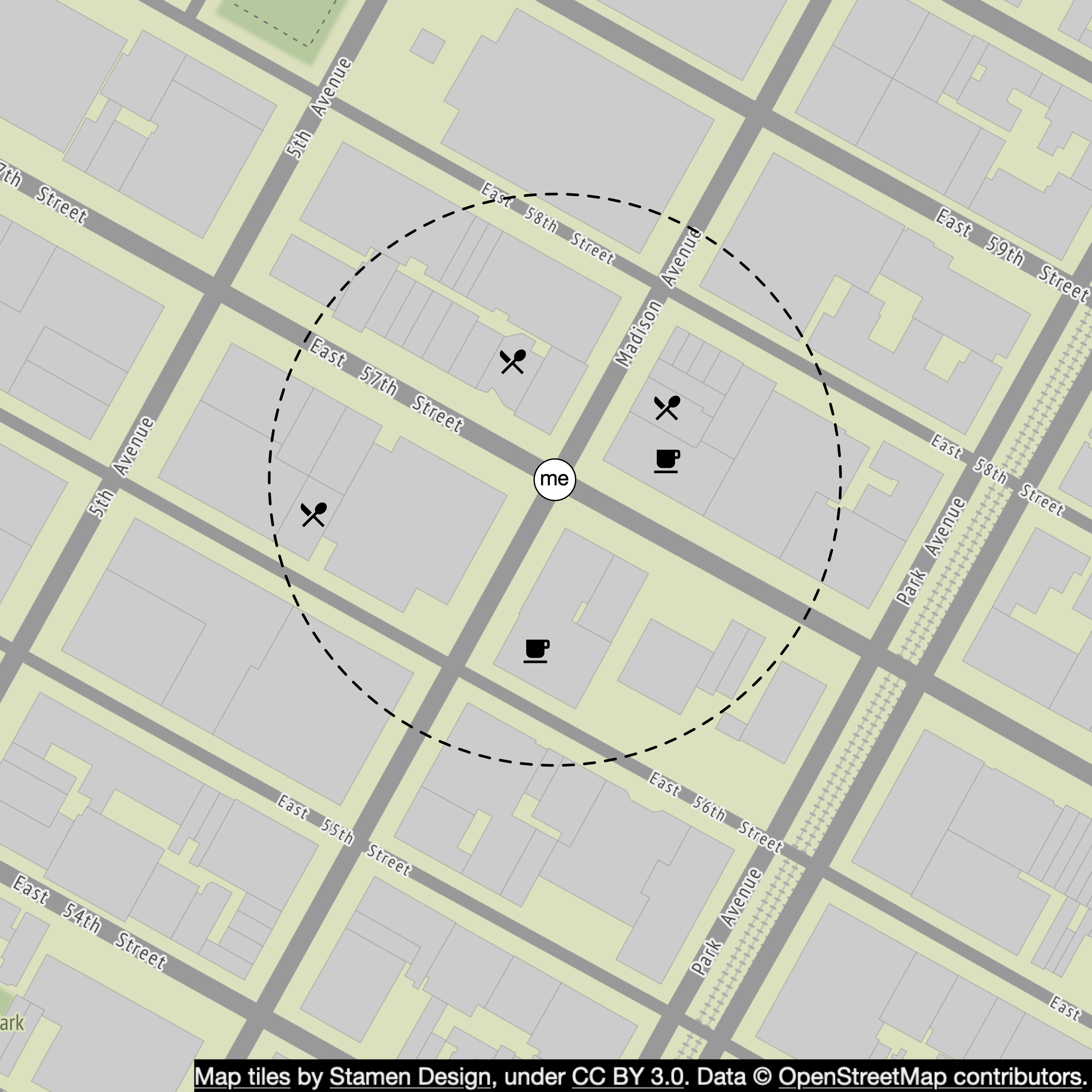

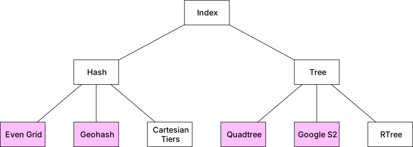
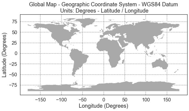
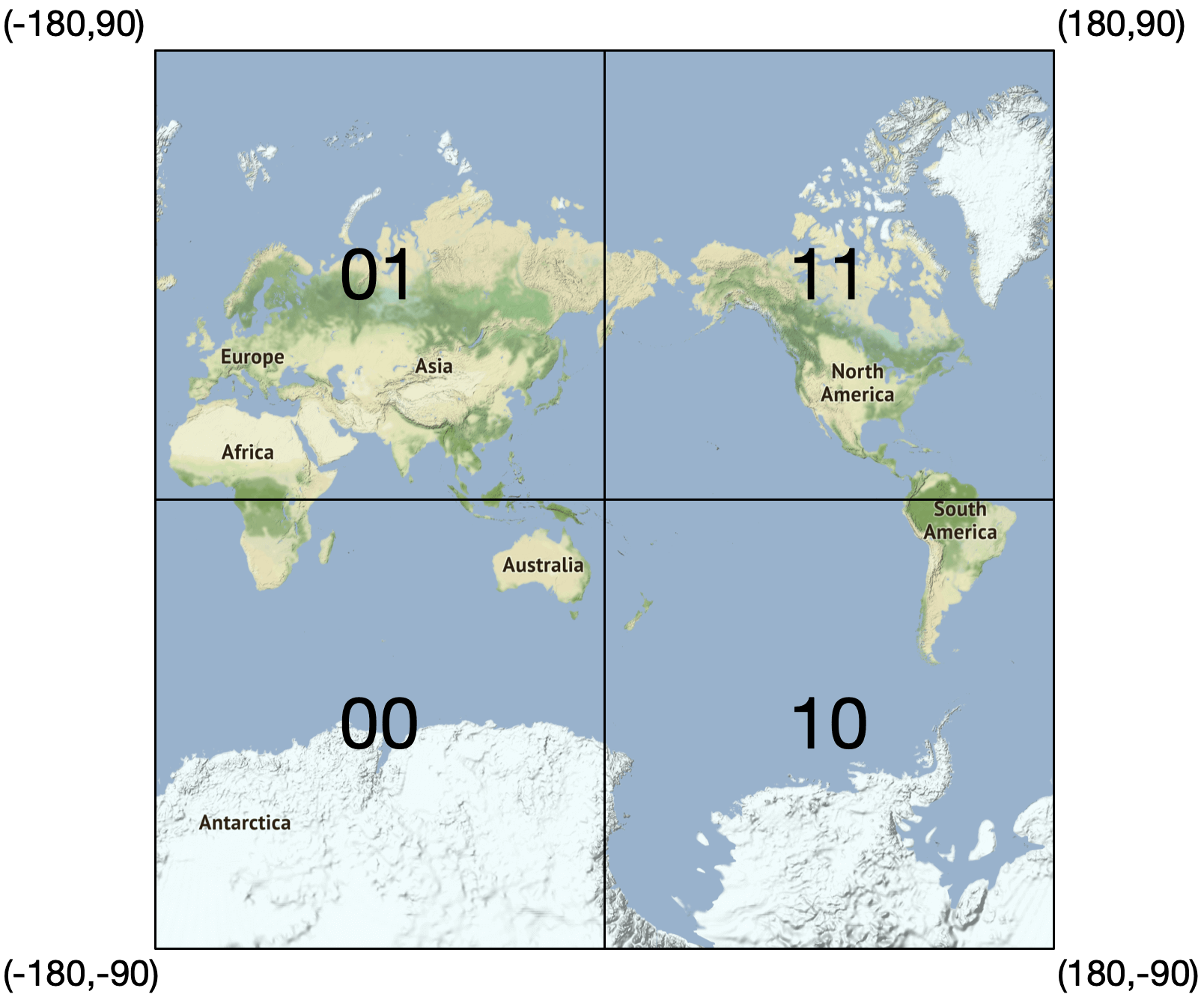
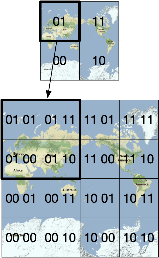
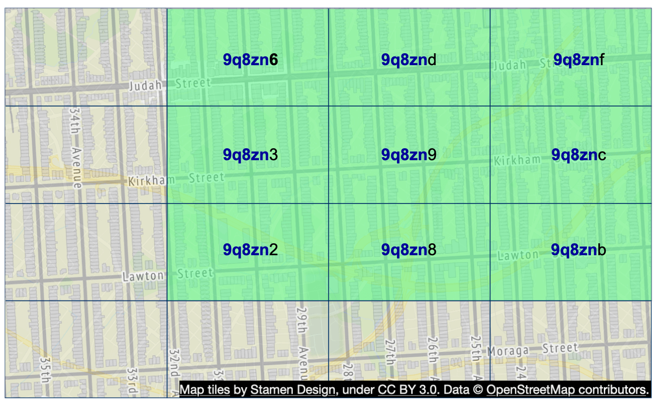
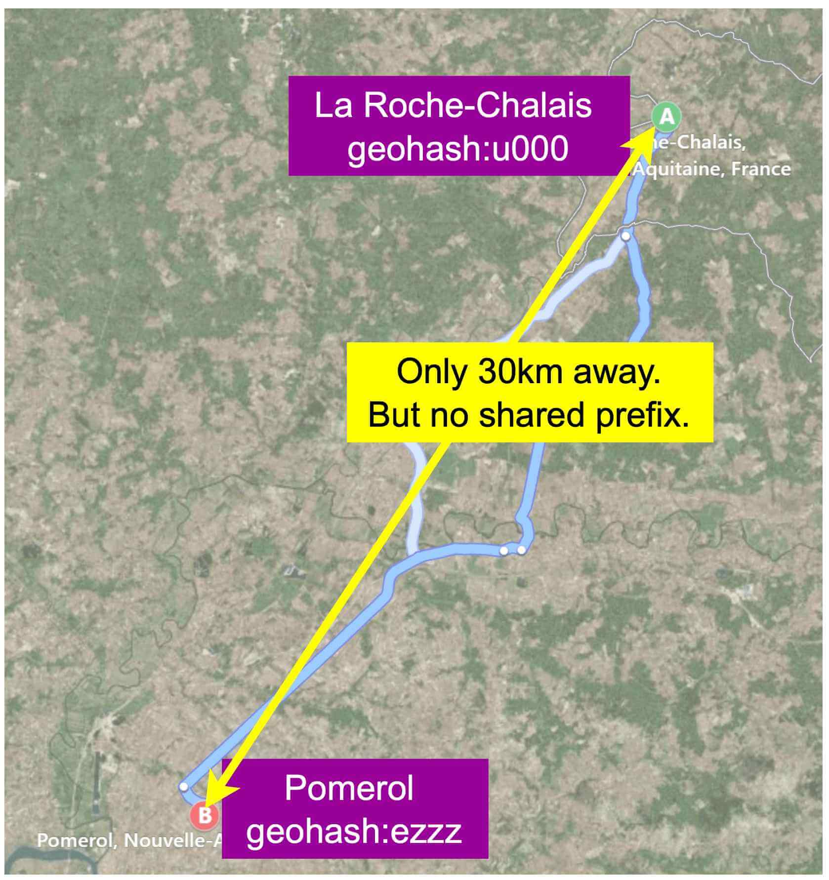
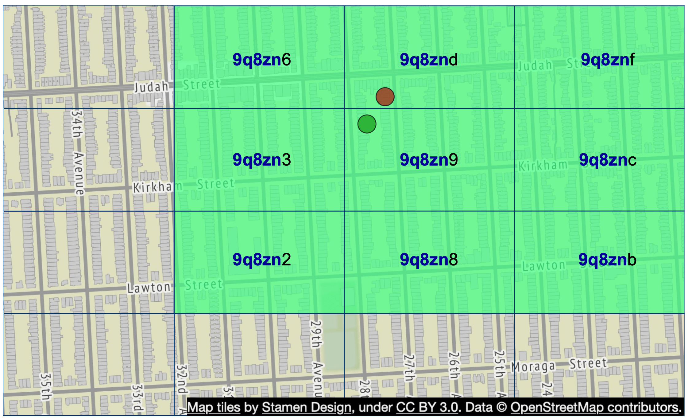
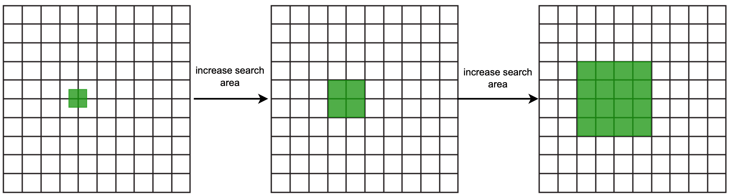
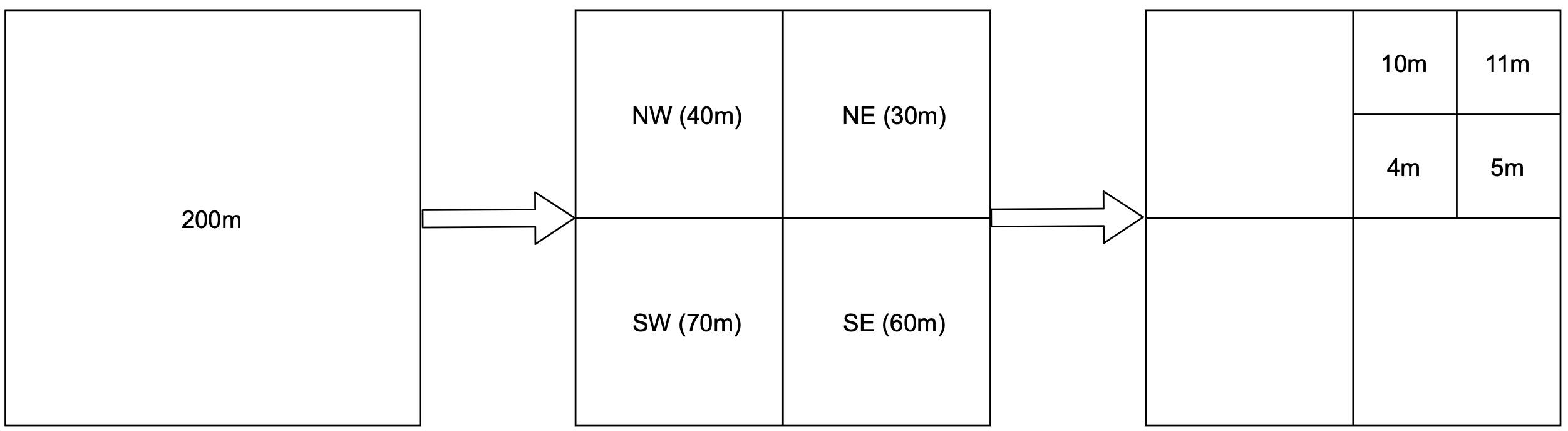
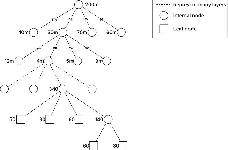
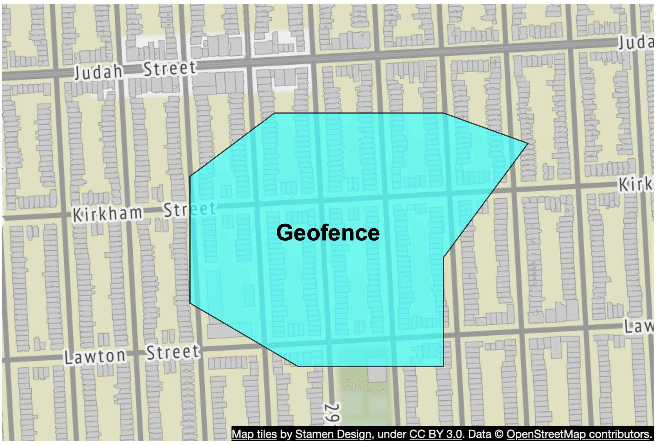
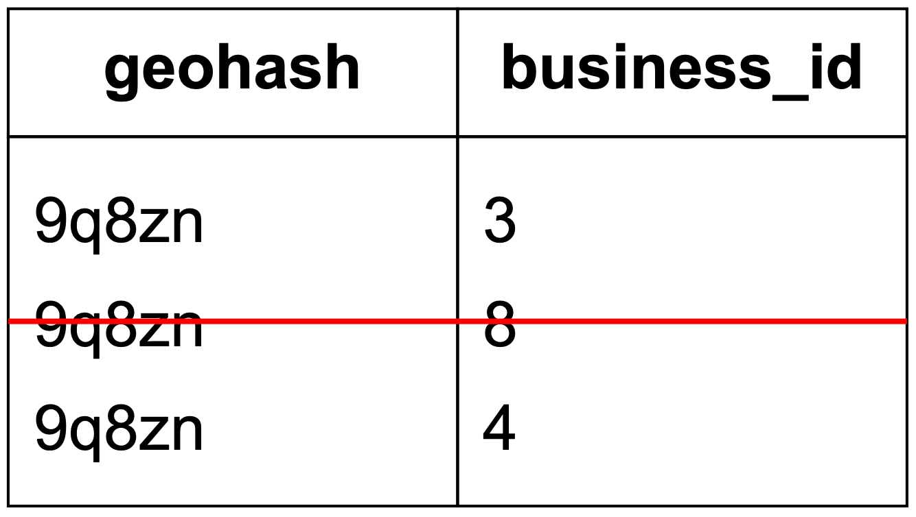
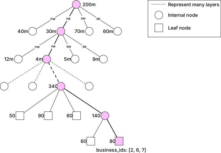
Step 3 - Design Deep Dive
Scale the database
**Business table:** Shard by business_id for even load distribution.
**Geospatial index table (geohash):** Two storage options: - Option 1: `geohash → JSON array of business_ids` (one row per geohash). - Option 2: `(geohash, business_id)` compound key — one row per business (Table 9, Table 10).
**Recommendation: Option 2** — simple addition/removal without locks, no duplicate scan needed.
**Scaling the geospatial index:** Full dataset is small (~1.71 GB for quadtree). Use read replicas instead of sharding (simpler to develop and maintain).
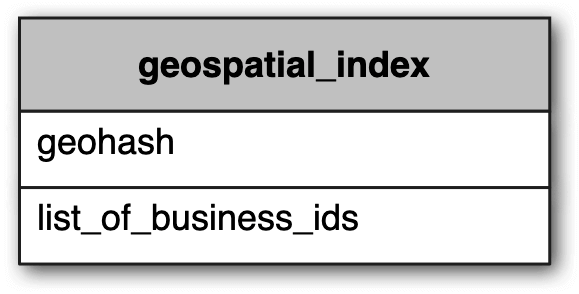
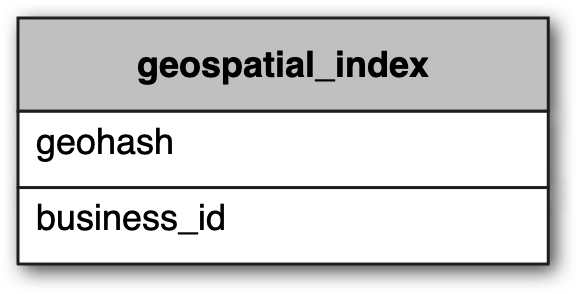
Caching
Cache considerations: workload is read-heavy but dataset is relatively small — may already fit in DB working set. Add read replicas first; cache if benchmarking shows need.
**Cache key:** Location coordinates are not reliable (GPS inaccuracy, slight movement). Use geohash as cache key — small location changes map to the same geohash.
**Two types of cached data (Table 12):** 1. `geohash → list of business IDs` — precomputed for each geohash precision (4, 5, 6). Total: ~5 GB (8 bytes × 200M businesses × 3 precisions). 2. `business_id → business object` — hydrated business data for rendering.
Deploy Redis cache globally (same copy) for low latency across regions.
Region and availability zones
Deploy LBS to multiple regions and availability zones (Figure 20): - Makes users physically closer to the system. - Flexible load distribution (Japan/Korea have high population density). - Privacy law compliance (some countries require data stored locally).
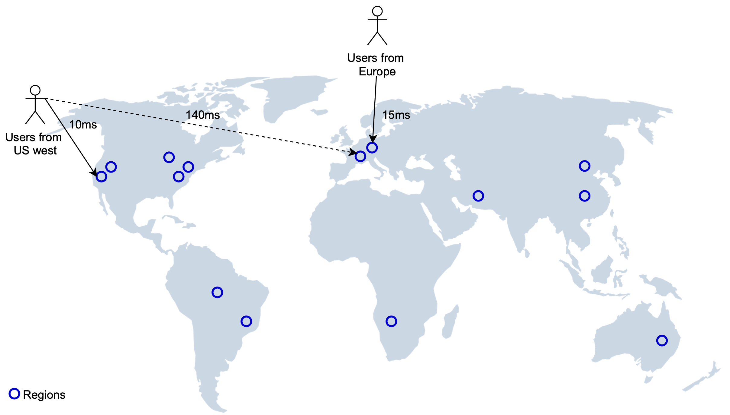
Final design diagram
Figure 21 shows the final design.
**Get nearby businesses flow:** 1. Client sends location (lat/long) and radius (e.g., 500m) to load balancer. 2. Load balancer forwards to LBS. 3. LBS looks up geohash length for 500m radius → length 6. 4. LBS calculates neighboring geohashes (8 neighbors + self). 5. LBS fetches business IDs from "Geohash" Redis cache for each geohash in parallel. 6. LBS fetches hydrated business objects from "Business info" Redis cache, calculates distances, ranks, and returns results.
**View/update/add/delete business:** - Business service first checks "Business info" Redis cache. - Cache miss → fetch from database and cache result. - Cached business data updated by nightly job (new/updated businesses effective next day).
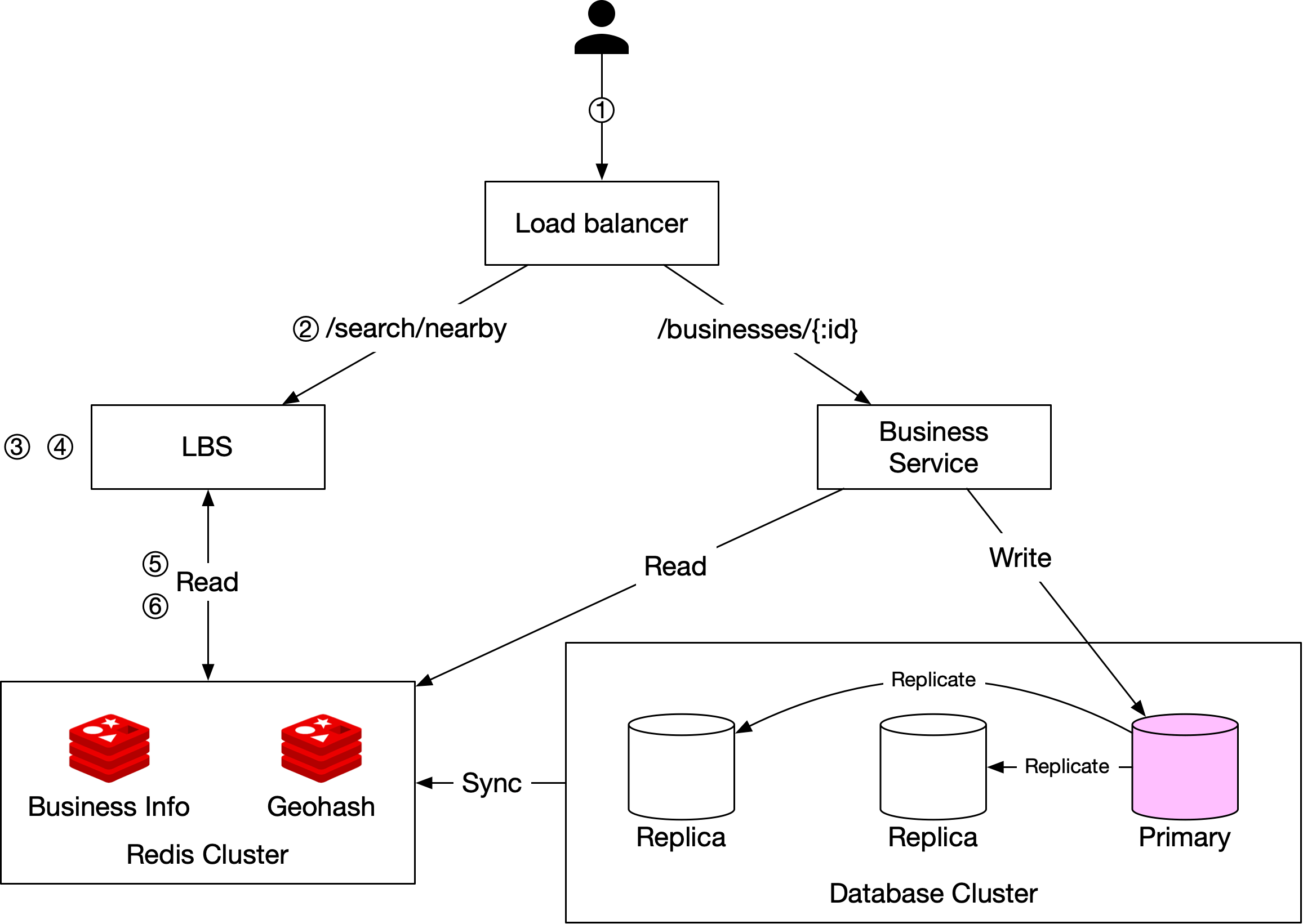
Step 4 - Wrap Up
We designed a proximity service using geospatial indexing (geohash). Key topics covered: - Five indexing options: 2D search, even grid, geohash, quadtree, Google S2. - Caching with geohash as cache key. - Database scaling via read replicas. - Multi-region deployment for availability and compliance.
Nearby Friends
We design a scalable backend for a "Nearby Friends" feature. For an opt-in user, the mobile client presents a list of friends who are geographically nearby. Unlike proximity services where business locations are static, user locations change frequently — requiring a dynamic, real-time design.
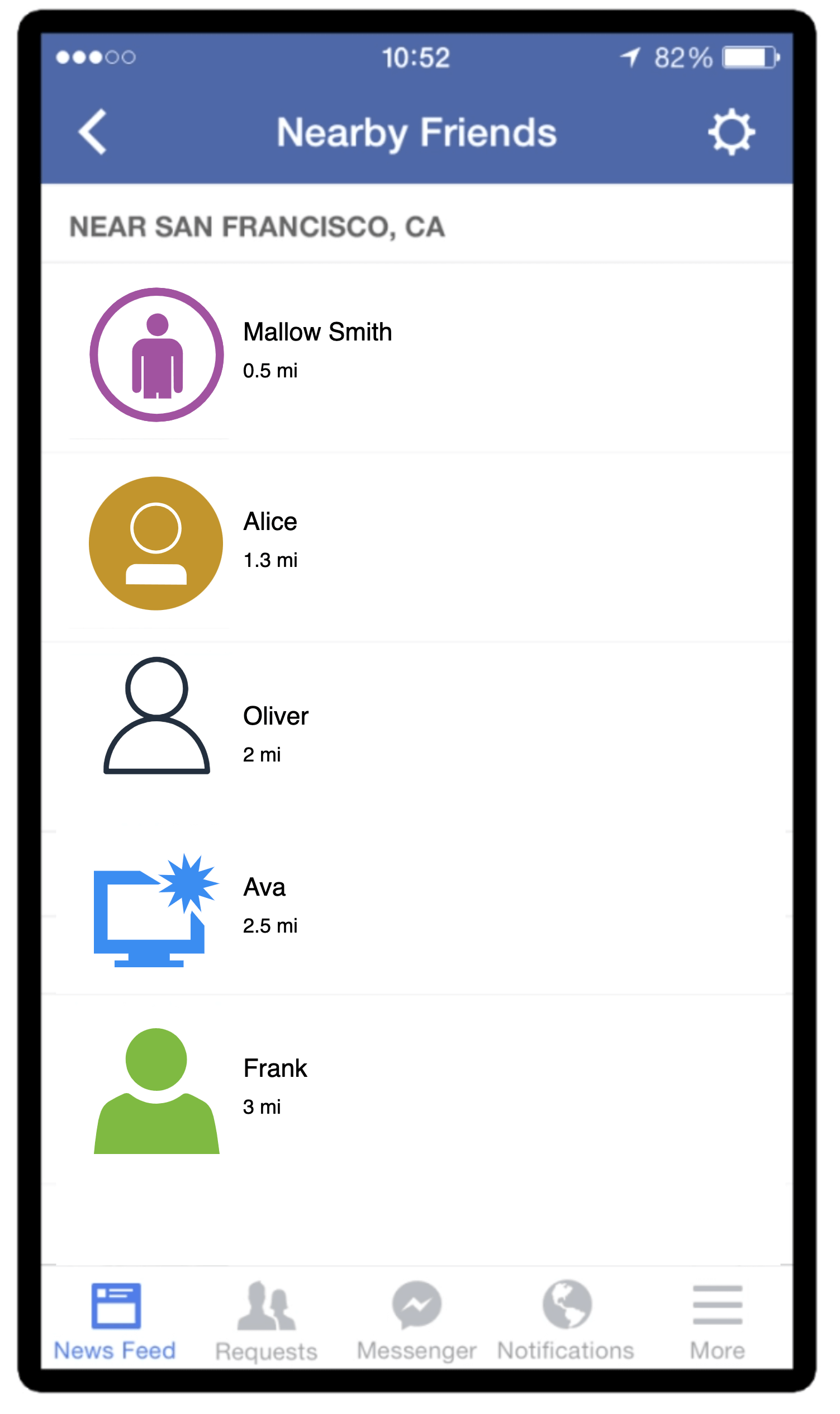
Step 1 - Understand the Problem and Establish Design Scope
**Functional requirements:** - Users see nearby friends on their mobile apps. - Each entry shows distance and timestamp of last update. - Nearby friend list updated every few seconds. - "Nearby" = within 5 miles (configurable). - Friends inactive for 10+ minutes disappear from list. - Store location history.
**Non-functional requirements:** - Low latency for location updates. - Reliability (occasional data point loss acceptable). - Eventual consistency (a few seconds delay acceptable).
**Back of the envelope estimation:** - 1 billion users; 10% use nearby friends = 100M DAU. - 10% concurrent users = 10M concurrent. - Location refresh interval: 30 seconds. - Average 400 friends, 10% online and nearby. - **Location update QPS = 10M / 30 ≈ 334,000 QPS** - Forwarding QPS = 334K × 400 × 10% = **14M location updates/second**
Step 2 - Propose High-Level Design and Get Buy-In
High-level design
Conceptually, a user could maintain peer-to-peer connections to all nearby active friends (Figure 2) — not practical for mobile devices (flaky connections, power consumption).
A shared backend (Figure 3) handles: - Receiving location updates from all active users. - Forwarding each update to all active friends within the radius. - Dropping updates for friends beyond the threshold.
Figure 4 shows the proposed design with these components:
- **Load balancer:** Distributes traffic across RESTful API servers and WebSocket servers. - **RESTful API servers:** Stateless HTTP servers for auxiliary tasks (add/remove friends, update profiles). - **WebSocket servers:** Stateful, bi-directional. Each client maintains one persistent WebSocket connection. Handles near-real-time location updates and initializes client with all nearby online friends' locations. - **Redis location cache:** Stores most recent location per active user with TTL. TTL refreshed on every update; expired = user inactive. - **User database:** User data and friendship data (relational or NoSQL). - **Location history database:** Historical location data (not directly used by nearby friends feature). - **Redis pub/sub server:** Lightweight message bus. Each user has a dedicated channel. WebSocket handlers subscribe to friends' channels and receive location updates.
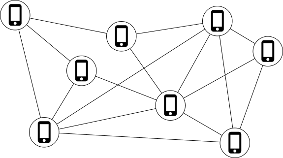
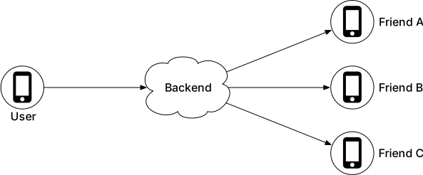
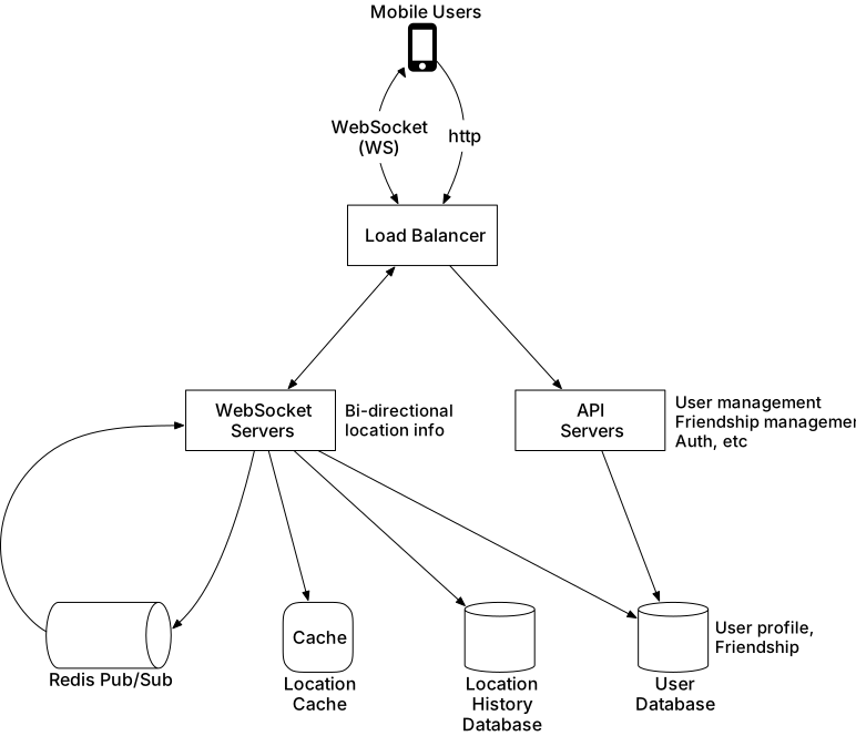
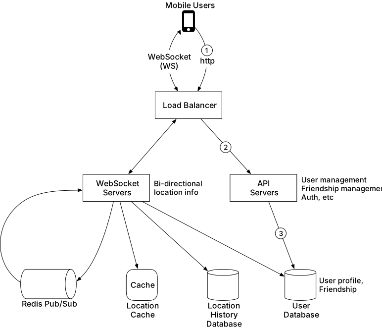
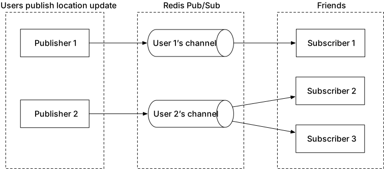
Periodic location update
Figure 7 shows the periodic location update flow: 1. Mobile client sends location update over persistent WebSocket connection. 2. Load balancer forwards to client's WebSocket server. 3. WebSocket server saves to location history database. 4. WebSocket server updates Redis location cache (refreshes TTL); stores location in connection handler variable. 5. WebSocket server publishes new location to user's channel in Redis pub/sub. 6. Redis pub/sub broadcasts to all subscribers (friends' WebSocket connection handlers). 7. Each receiving WebSocket handler computes distance between the update sender and the subscriber. 8. If distance ≤ search radius, send location + timestamp to subscriber's client. Otherwise, drop.
Figure 8 shows a concrete example with users 1-6.
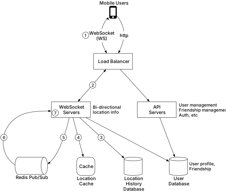
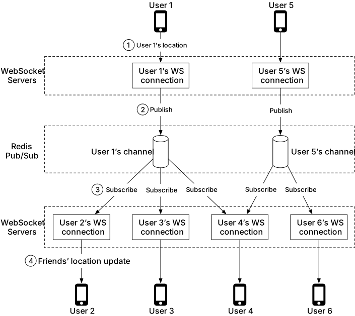
API design
**WebSocket APIs:** 1. Periodic location update: send latitude, longitude, timestamp. 2. Receive location updates: receive friend location data + timestamp. 3. WebSocket initialization: send location; receive all nearby friends' locations. 4. Subscribe to new friend: send friend_id; receive latest location. 5. Unsubscribe a friend: send friend_id.
**Data model:** - **Location cache (Redis):** `user_id → {latitude, longitude, timestamp}` with TTL. - Redis chosen for fast read/write, TTL support, no need for durable storage. - **Location history database (Cassandra):** `user_id, latitude, longitude, timestamp`. - Heavy-write workload; horizontally scalable by sharding on user_id.
Step 3 - Design Deep Dive
Scaling WebSocket servers
WebSocket servers are stateful — before removing a node, mark it as "draining" at the load balancer (no new connections routed to it). Once existing connections close, remove the server.
**Client initialization:** On WebSocket connection start: 1. Update user location in Redis cache. 2. Store location in connection handler variable. 3. Load all friends from user database. 4. Batch-fetch locations from Redis cache. 5. For each friend within radius, return profile, location, timestamp to client. 6. Subscribe to all friends' pub/sub channels (even inactive — they use no CPU, minimal memory). 7. Publish user's current location to their own pub/sub channel.
Scaling Redis pub/sub servers
**Memory usage:** 100M channels × 20 bytes × 100 friends = ~200 GB total. Need ~2 Redis servers (100 GB each).
**CPU usage:** 14M pushes/sec ÷ 100K pushes/server ≈ **140 Redis servers** needed.
Bottleneck is CPU, not memory. Need a distributed Redis pub/sub cluster.
**Distributed pub/sub cluster:** Shard channels across hundreds of Redis servers using consistent hashing (Figure 9). Use a service discovery component (etcd or Zookeeper) to store the hash ring and notify WebSocket servers of changes.
Figure 10 shows how a WebSocket server finds the correct pub/sub server for a user's channel.
**Scaling considerations:** - Pub/sub channels are stateless (messages not persisted), but subscriber lists are stateful. - Treat pub/sub cluster like a stateful storage cluster — scale carefully. - Over-provision to handle daily peak. Resize only during lowest-usage periods. - On resize: hash ring update triggers mass resubscription — monitor WebSocket CPU spike.
**Replacing a failed pub/sub server (Figure 11):** - Update hash ring in service discovery with new node replacing failed one. - WebSocket servers re-subscribe affected channels to the new server.
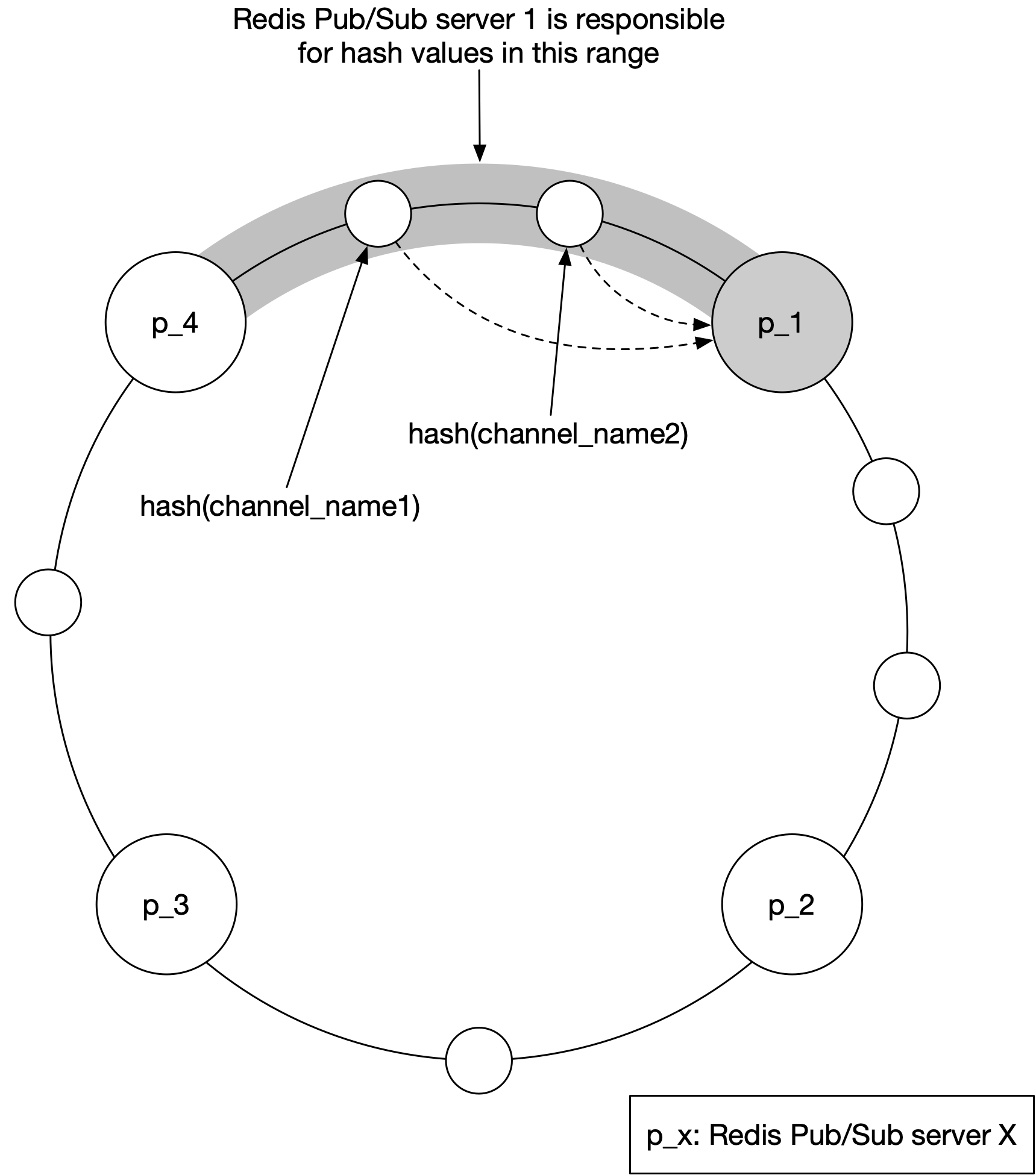
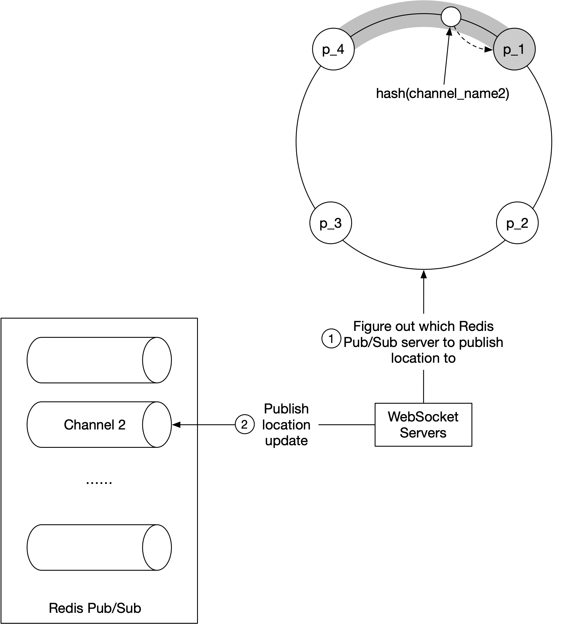
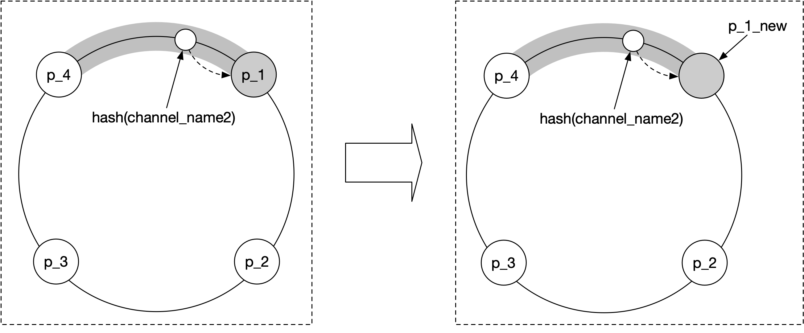
Nearby random person (bonus)
To show random opt-in users (not just friends): add a pool of pub/sub channels by geohash (Figure 12). Anyone within a grid subscribes to the same channel.
Figure 13: When user 2 updates location, WebSocket handler computes geohash and publishes to that channel. All nearby subscribers (excluding sender) receive the update.
Figure 14: Each client subscribes to their current geohash and 8 surrounding geohash grids to handle border cases.

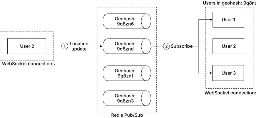
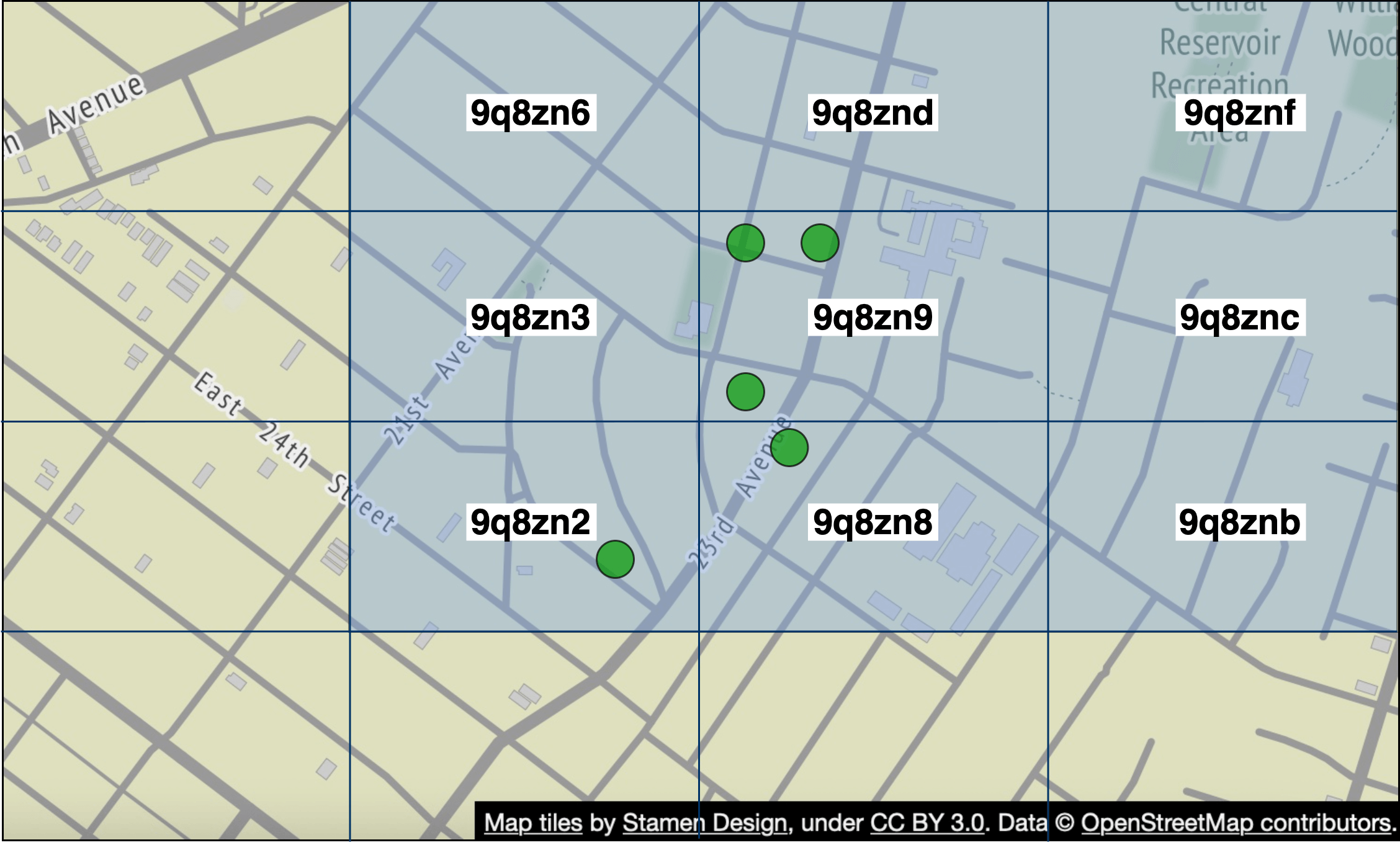
Alternative to Redis pub/sub
**Erlang/Elixir (BEAM VM + OTP):** Better solution for this problem. - Lightweight Erlang processes (~300 bytes each) — can model each user as a process. - 10M processes easily on modern servers. - Native inter-process messaging and subscription via OTP. - Forms a mesh for efficiently routing updates from one user to many friends. - Excellent distributed operations and debugging tools. - Trade-off: niche technology, harder to hire for.
Step 4 - Wrap Up
Core components: WebSocket (real-time), Redis location cache (fast read/write with TTL), Redis pub/sub (routing layer). Key challenges addressed: 14M location updates/second, stateful WebSocket scaling with draining, distributed pub/sub cluster with consistent hashing.
Google Maps
We design a simplified version of Google Maps — a web mapping service providing satellite imagery, street maps, real-time traffic conditions, and route planning. As of March 2021, Google Maps had 1 billion DAU, 99% world coverage, and 25 million daily updates. Features in scope: location update, navigation, ETA, and map rendering. Map tiles in this chapter are from Stamen Design; data from OpenStreetMap.
Step 1 - Understand the Problem and Establish Design Scope
**Key requirements:** - 1 billion DAU. - Features: location update, navigation, ETA, and map rendering. - Support multiple travel modes (driving, walking, bus). - Take traffic conditions into consideration. - No multi-stop directions, no business places/photos.
**Non-functional requirements:** - Accuracy: users must not be given wrong directions. - Smooth navigation: smooth map rendering on client-side. - Data and battery usage: minimize for mobile devices. - High availability and scalability.
Map 101
**Positioning system:** - Latitude: how far north or south. - Longitude: how far east or west.
Figure 1 shows the latitude/longitude coordinate system.
**Going from 3D to 2D (Map Projection):** Translating points from a 3D globe to a 2D plane is called Map Projection. Every projection distorts actual geometry. Google Maps uses Web Mercator (modified Mercator projection). Figure 2 shows several projection examples.
**Geocoding:** Converting addresses to geographic coordinates (and reverse geocoding — lat/lng back to human-readable address). One method: interpolation using GIS data.
**Geohashing (Figure 3):** Encodes a geographic area into a short string. Recursively divides earth into sub-grids. Used in our design for map tiling.
**Map rendering:** The world is broken into smaller tiles. The client downloads only relevant tiles for the current area/zoom level and stitches them together. Different tile sets exist for different zoom levels — client chooses appropriate set.
**Road data processing for navigation algorithms:** Routing algorithms (Dijkstra's, A*) operate on a graph where intersections are nodes and roads are edges (Figure 4). The world graph is too large for memory — broken into routing tiles using geohash-based subdivision. Each routing tile contains nodes/edges for its geographic area and references to neighboring tiles. Hierarchical routing tiles (3 levels): local roads (small tiles), arterial roads (medium tiles), major highways (large tiles) — shown in Figures 5 and 6.
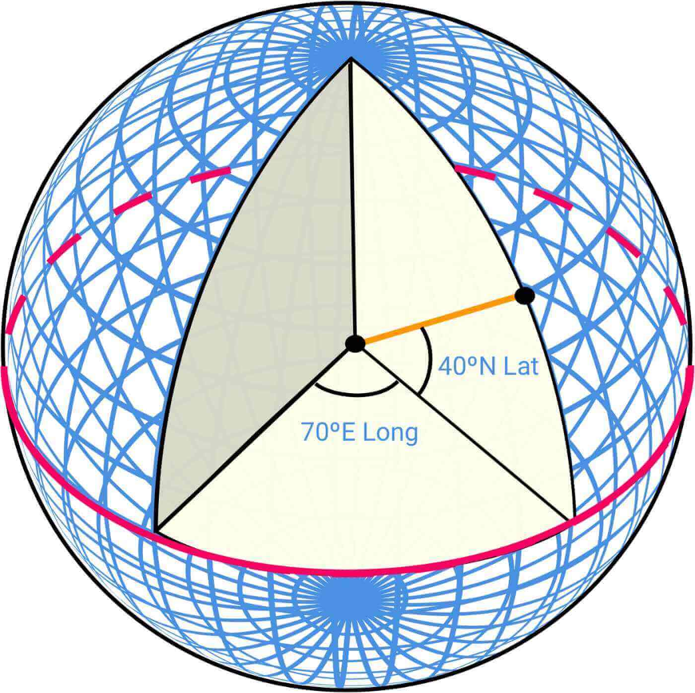

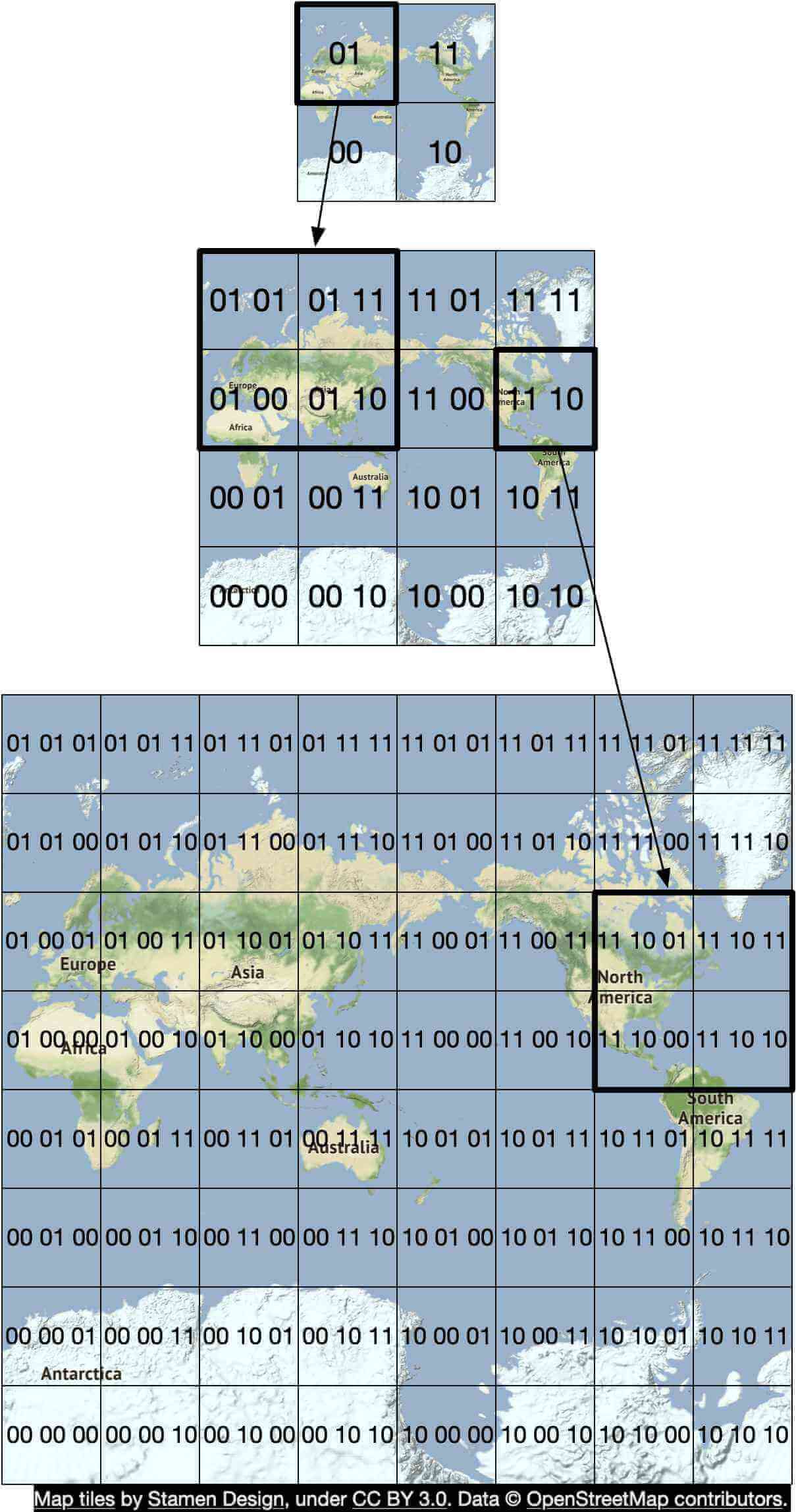
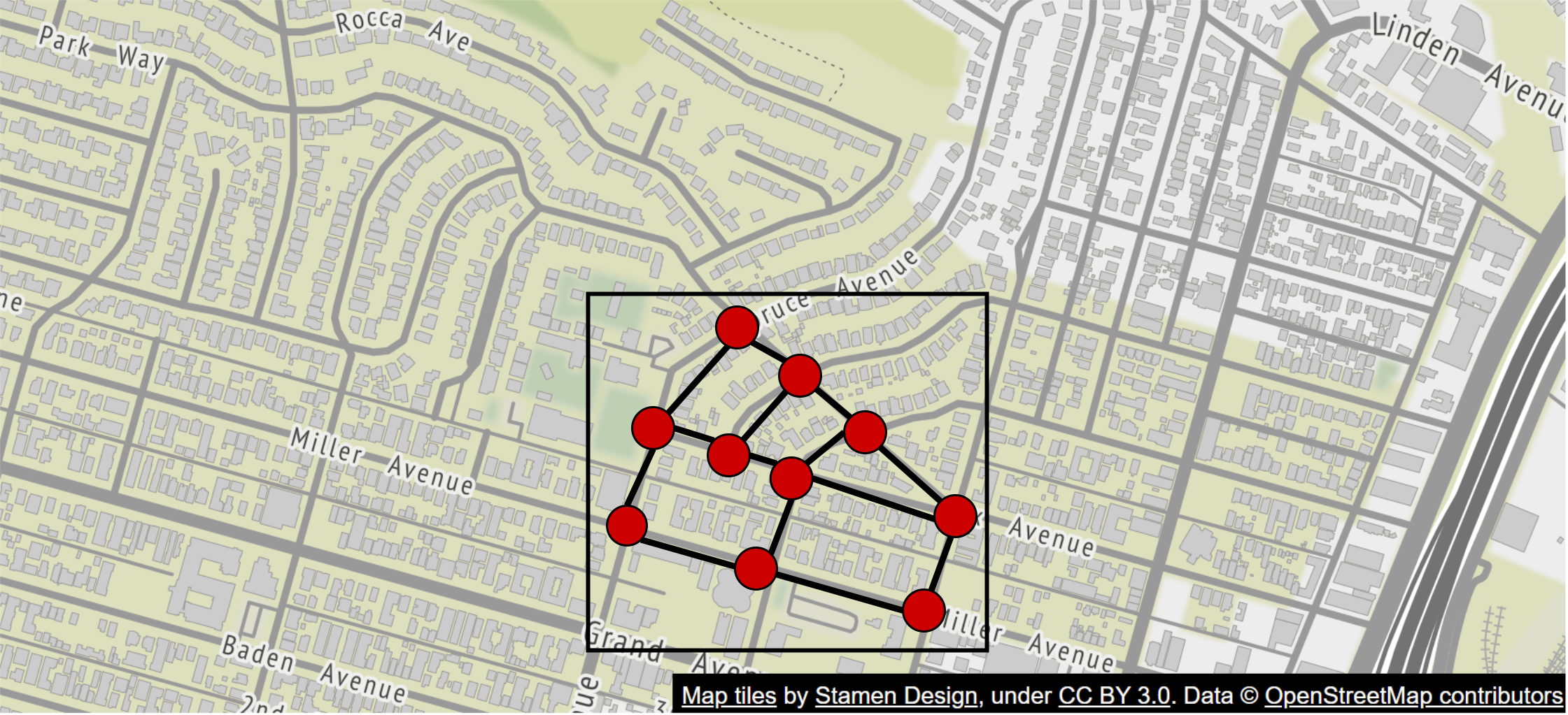

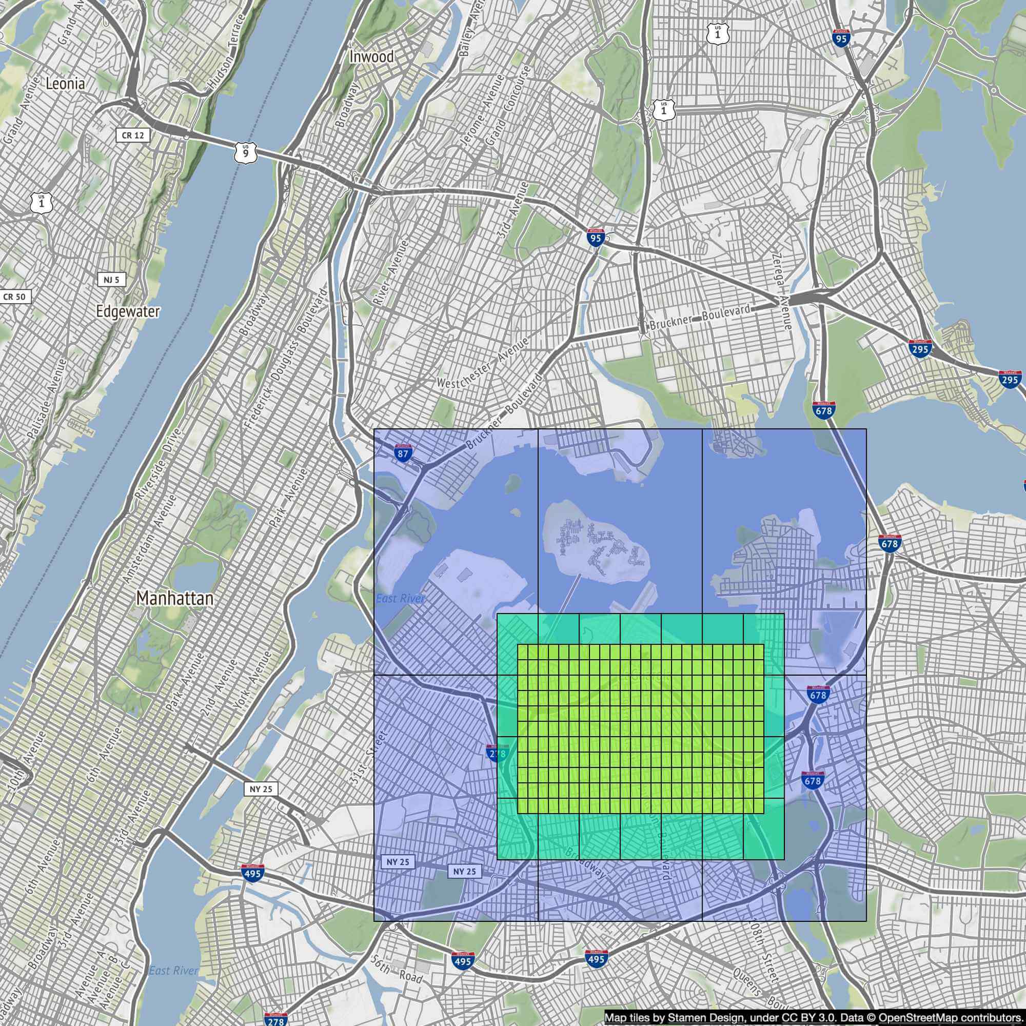
Back-of-the-envelope estimation
**Storage usage:** - At zoom level 21: ~4.4 trillion tiles × 100 KB = 440 PB. - 90% of world surface is highly compressible (oceans, deserts) → reduce by 80-90% → **~50 PB** for highest zoom level. - Total across all zoom levels (geometric series): **~100 PB**. - Road data: TBs of raw data from external sources → routing tiles also TBs.
**Server throughput (location updates):** - 1B DAU × 35 min/week navigation = 5B min/day. - GPS update every second → 300B req/day = 3M QPS. - Batch every 15 seconds → **200,000 QPS** average. - Peak QPS = 200,000 × 5 = **1 million QPS**.
**CDN data usage:** - At 30 km/h, each 200m×200m tile = 100 KB → 1.25 MB/min. - 5B nav minutes/day × 1.25 MB = 6.25 billion MB/day → 62,500 MB/sec. - 200 CDN POPs → ~300 MB/sec per POP.
Step 2 - Propose High-Level Design and Get Buy-In
High-level design
Figure 7 shows the high-level design with three core services: location service, navigation service, and map rendering.
**Location service (Figure 8):** Clients send batched location updates every 15 seconds (buffered locally, reducing QPS from 3M to 200K). Protocol: HTTP with keep-alive. ``` POST /v1/locations Parameters: locs — JSON array of (latitude, longitude, timestamp) tuples ``` Database needs high write throughput and horizontal scalability → Cassandra. Also log to Kafka stream for downstream services.
**Navigation service:** Finds reasonably fast route from A to B. Tolerates slight latency; accuracy is critical. ``` GET /v1/nav?origin=1355+market+street,SF&destination=Disneyland ``` Returns distance, duration, HTML instructions, polyline, travel mode.
**Map rendering:** Client fetches tiles on-demand. Two options: - Option 1: Generate tiles dynamically → heavy server load, hard to cache. Not recommended. - Option 2: Pre-generated static tiles at each zoom level, served via CDN (Figure 10).
Figure 11 shows CDN POPs serving tiles globally — clients fetch from nearest POP.
Tile URL uses geohash: `https://cdn.map-provider.com/tiles/9q9hvu.png`
Alternative rendering flow (Figure 12): Instead of hardcoding geohash algorithm on client, a map tile service translates (location, zoom level) → 9 tile URLs (current + 8 surrounding). Client then fetches from CDN.
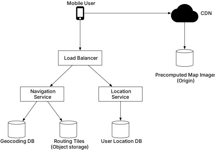
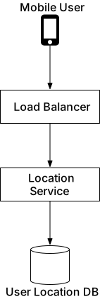
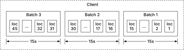
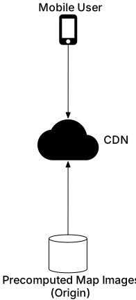
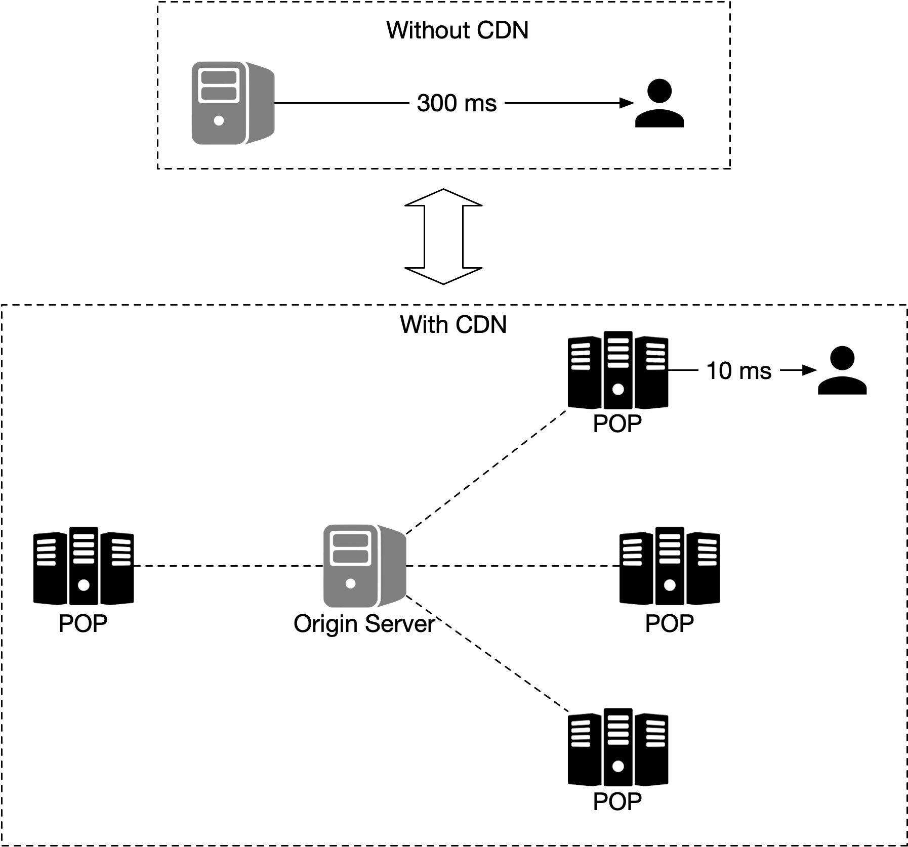
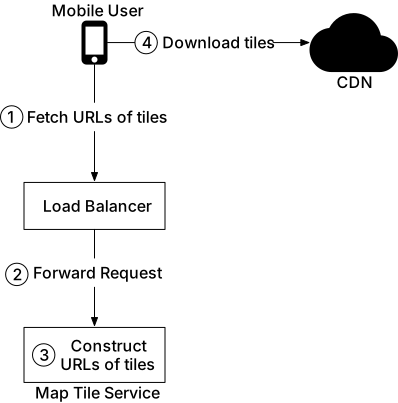
Step 3 - Design Deep Dive
Data model
Four types of data:
**Routing tiles:** Generated by an offline routing tile processing service from raw road datasets. Three resolution levels (local roads, arterial roads, highways). Stored as binary adjacency lists in object storage (S3), organized by geohash for fast lookup. Cached aggressively by routing services.
**User location data (Figure 14):** High write volume → Cassandra. Schema: `(user_id, timestamp) → (lat, lng, user_mode, navigation_mode)`. `user_id` as partition key; `timestamp` as clustering key for efficient range reads.
**Geocoding database:** Converts addresses/place names to lat/lng. Key-value store (Redis) for fast reads (frequent reads, infrequent writes).
**Precomputed map tiles:** PNG images at 21 zoom levels. Stored in CDN backed by S3. Encoded by geohash for easy lookup.
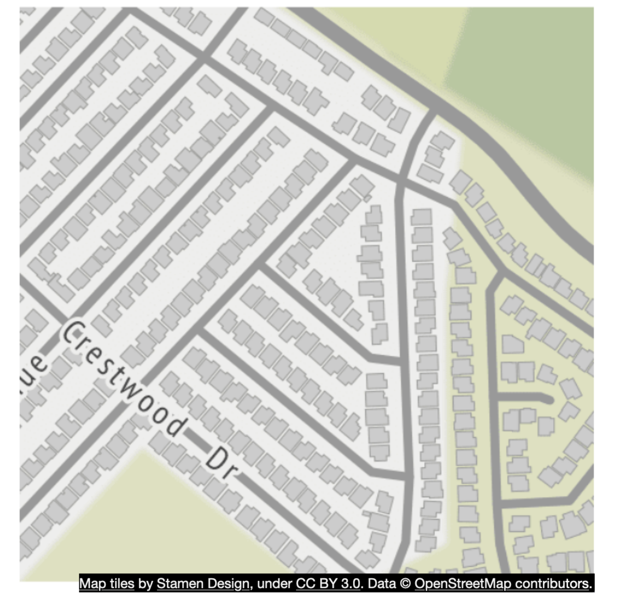
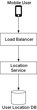
Location service (deep dive)
Location data is logged to Kafka in addition to being written to Cassandra. Downstream services consume the Kafka stream (Figure 15): - **Live traffic service:** extracts traffic conditions → updates live traffic database. - **Routing tile processing service:** detects new/closed roads → updates routing tiles in S3. - Other services for analytics, personalization, etc.
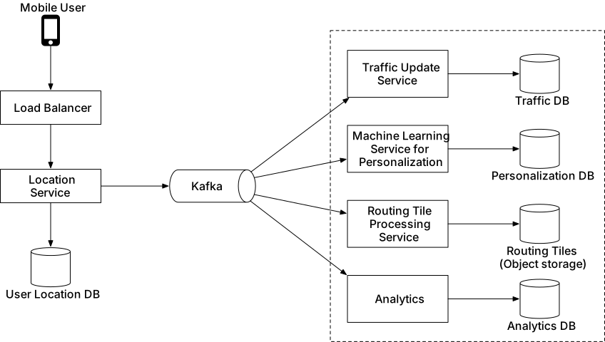
Map rendering (deep dive)
Google Maps uses 21 zoom levels (Figure 16): - Level 0: entire world in one 256×256px tile. - Each zoom level: tiles double in both directions (4× total tiles per level). - Level 21: ~4.4 trillion tiles.
**Vector tiles (future improvement):** Instead of PNG images, send vector data (paths/polygons). Benefits: - Vector data compresses much better than images. - Smoother zooming — vectors scale cleanly without pixelation (WebGL-based rendering).
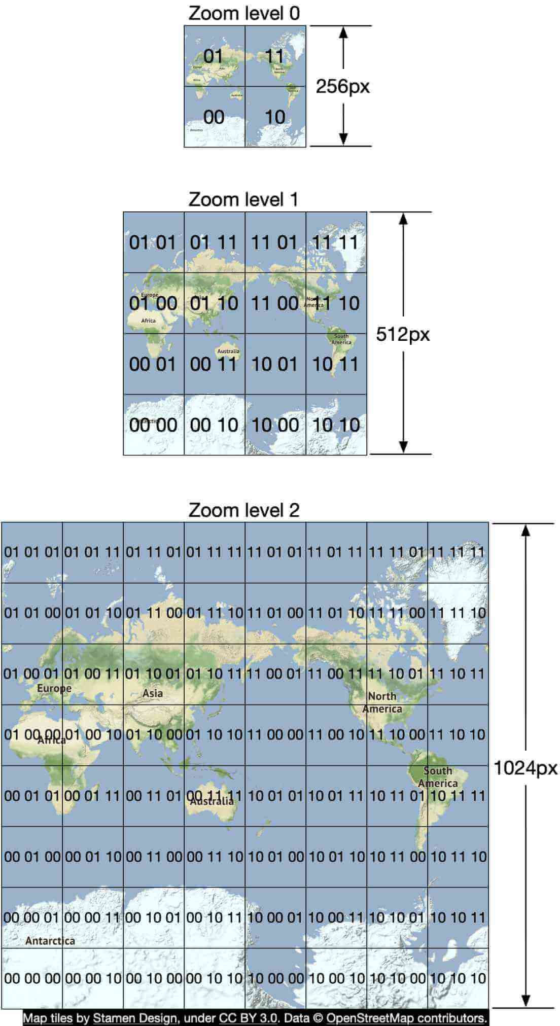
Navigation service (deep dive)
Figure 17 shows the full navigation service design. Components:
1. **Geocoding service:** Converts address/place name → lat/lng pair. 2. **Route planner:** Orchestrates the routing pipeline. Calls shortest-path service, gets ETA predictions, passes to ranker. 3. **Shortest-path service:** Runs A* variation against routing tiles in S3. Algorithm: - Convert origin/destination lat/lng → geohashes → load routing tiles. - Traverse graph, hydrate neighboring tiles from S3 on-demand. - Traverse between tile resolution levels (local → arterial → highway) via cross-tile connections. - Figure 18 shows conceptual graph traversal across tiles. 4. **ETA service:** Predicts ETAs using ML on current traffic + historical data, including future traffic prediction. 5. **Ranker service:** Applies user filters (avoid tolls, avoid freeways), ranks routes fastest to slowest. 6. **Updater services (async):** - Routing tile processing service: detects road changes from location stream. - Traffic update service: extracts live traffic from location stream → live traffic database.
**Adaptive ETA and rerouting (Figure 19, 20):** Server tracks actively navigating users. Naive approach: store routes as lists of routing tiles, O(n×m) scan for affected users.
Optimized approach: for each user, store hierarchical chain of routing tiles — current tile + its parent tile + grandparent... until destination is covered. To check if user is affected by a traffic change in tile T, only check if T is contained in the last (largest) tile in the user's chain. This quickly filters most users.
Periodically recalculate ETAs for all active navigating users; notify if a faster route is found.
**Delivery protocol:** WebSocket chosen over SSE or long polling — supports bi-directional communication for rerouting and last-mile delivery.
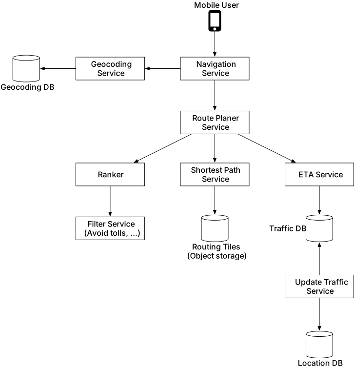
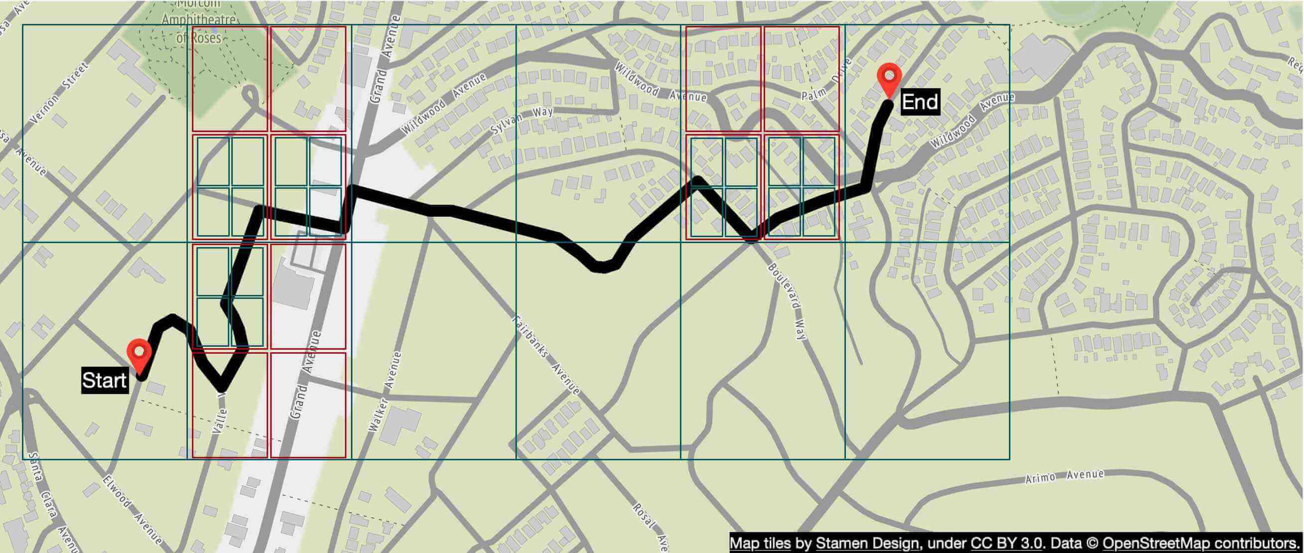
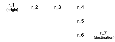
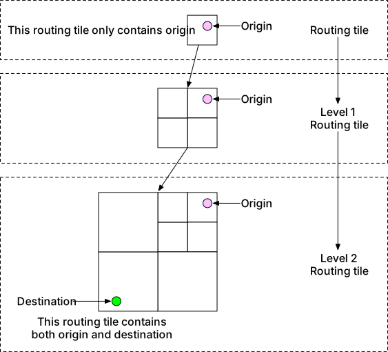
Step 4 - Wrap Up
We designed a simplified Google Maps with location update, ETAs, route planning, and map rendering. Key components: Cassandra for high-write location data, Kafka for event streaming, CDN for precomputed map tiles, hierarchical routing tiles in S3, A* pathfinding with on-demand tile hydration.
Figure 21 shows the final design integrating all components.
Potential extension: multi-stop navigation for delivery services (Doordash, Uber, Lyft) — find optimal order to visit destinations with live traffic awareness.
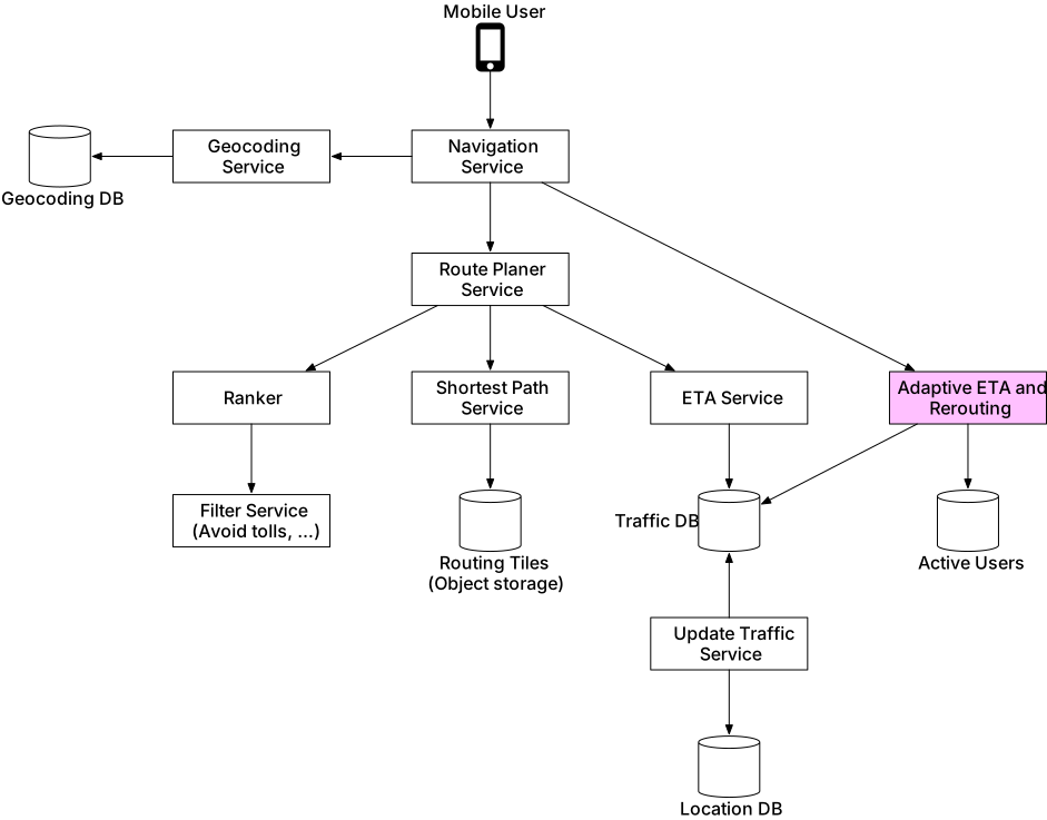
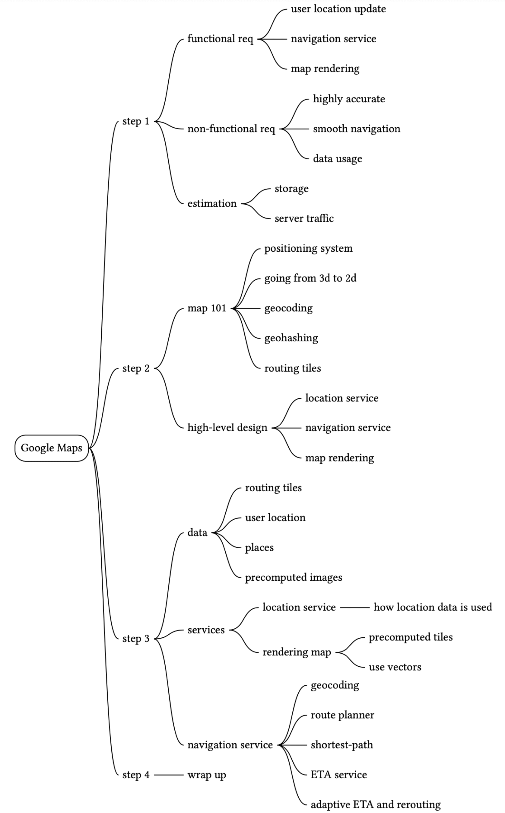
Distributed Message Queue
We design a distributed message queue — a system that provides communication and coordination between independent building blocks. Benefits: decoupling (tight coupling eliminated), improved scalability (scale producers/consumers independently), increased availability (other components continue when one goes offline), better performance (async communication).
Figure 1 shows popular distributed message queues. Note: Kafka and Pulsar are technically event streaming platforms, but our design includes streaming features (long data retention, repeated consumption) often found only in those systems.
Step 1 - Understand the Problem and Establish Design Scope
**Functional requirements:** - Producers send messages to a message queue. - Consumers consume messages from a message queue. - Messages can be consumed repeatedly or only once. - Historical data can be truncated (2-week retention). - Message size: kilobyte range, text only. - Ordered delivery (same order as produced). - Configurable data delivery semantics: at-least-once, at-most-once, exactly-once.
**Non-functional requirements:** - High throughput or low latency (configurable by use case). - Scalable: distributed, supports sudden surge in volume. - Persistent and durable: data on disk, replicated across nodes.
**Note for traditional queues:** RabbitMQ-style queues don't persist messages long-term and don't guarantee ordering. Removing these requirements greatly simplifies the design.
Step 2 - Propose High-Level Design and Get Buy-In
Messaging models
**Point-to-point (Figure 3):** A message is consumed by exactly one consumer and removed from the queue after acknowledgment. No data retention.
**Publish-subscribe (Figure 4):** Messages sent to a topic are received by all subscribed consumers. Our design supports both models — pub-sub via topics, point-to-point simulated via consumer groups.

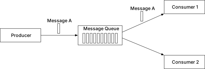
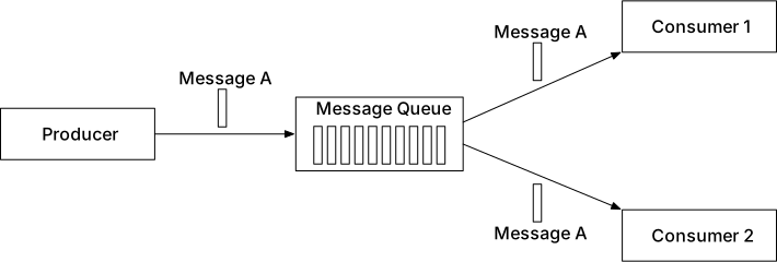
Topics, partitions, and brokers
**Partitions (Figure 5):** Topic data is sharded into partitions distributed across brokers. Each partition is a FIFO queue — maintains message order within the partition. Message position = offset.
Message routing: if message key is set → hash(key) % numPartitions; otherwise random partition.
**Message queue cluster (Figure 6):** Brokers hold partitions. Scaling a topic = increasing partition count.
**Consumer group (Figure 7):** - A set of consumers working together on topics. - Each group maintains its own consumed offsets. - Key constraint: a single partition can only be consumed by ONE consumer within a group → guarantees partition-level ordering. - If consumers > partitions, some consumers get no data. - Point-to-point simulation: put all consumers in same group.


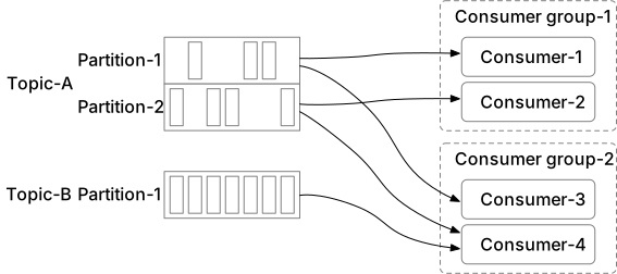
High-level architecture
Figure 8 shows the high-level design:
**Clients:** - Producer: pushes messages to specific topics. - Consumer group: subscribes and consumes messages.
**Core service and storage:** - Broker: holds multiple partitions. - Data storage: messages persisted in partitions. - State storage: consumer states (offsets, partition-consumer mapping). - Metadata storage: topic configuration (partition count, retention, replica distribution). - Coordination service (Zookeeper/etcd): service discovery (alive brokers), leader election (active controller that assigns partitions).
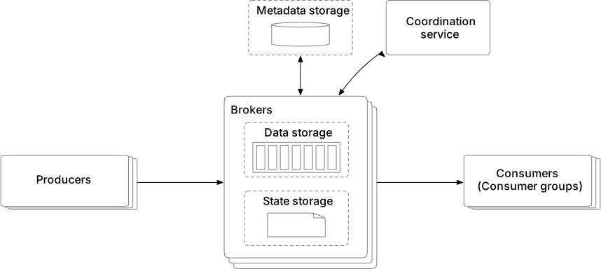
Step 3 - Design Deep Dive
Three key design choices for high throughput with high data retention: 1. On-disk data structure leveraging sequential access performance. 2. Message data structure with no-copy transit (producer → queue → consumer). 3. Favor batching everywhere (producer, broker, consumer).
Data storage
**Traffic pattern:** write-heavy, read-heavy; no updates/deletes; sequential read/write.
**Option 1 — Database:** Relational or NoSQL — not ideal. Hard to design for both heavy write and read at scale.
**Option 2 — Write-Ahead Log (WAL):** Append-only log file. Used in MySQL redo log, ZooKeeper WAL.
New messages appended to partition tail with monotonically increasing offset (Figure 9). Files divided into segments — only active segment receives writes. Non-active segments serve reads. Old segments truncated on retention/capacity limit.
Figure 10 shows segment files organized in `Partition-{:partition_id}` folders.
**Disk performance note:** Common misconception that disks are slow — true for random access only. Sequential access on modern RAID disks achieves several hundred MB/sec. OS also aggressively caches disk data in memory (WAL benefits heavily).
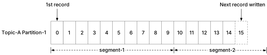
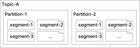
Message data structure
Schema: `key (byte[]), value (byte[]), topic (string), partition (int), offset (long), timestamp (long), size (int), crc (int)`
- **Key:** determines partition (hash(key) % numPartitions). Not unique — different from KV store keys. - **Value:** payload — plain text or compressed binary. - **Offset:** position in partition. Message found by (topic, partition, offset). - **CRC:** cyclic redundancy check for data integrity. - Optional fields (e.g., tags) can be added for filtering.
Producer flow
**Initial design (Figure 11):** Separate routing layer reads replica distribution from metadata, routes to leader replica broker.
Drawbacks: extra network hop, no batching.
**Improved design (Figure 12):** Routing layer + buffer integrated into producer client library. - Benefits: fewer network hops → lower latency, custom partition logic, batching for higher throughput.
**Batch size tradeoff (Figure 13):** Large batch → higher throughput, higher latency. Small batch → lower latency, lower throughput. Configurable per use case.
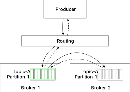
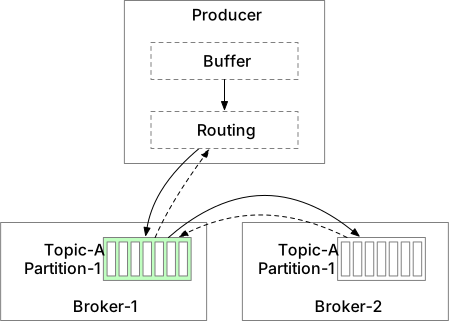

Consumer flow
Consumer specifies offset in a partition and receives a chunk of messages from that position (Figure 14).
**Push vs pull:** - Push: low latency but can overwhelm consumers; broker controls rate. - **Pull (chosen):** consumers control rate; suitable for batch processing; supports long polling to avoid wasted polling when no messages.
**Pull model workflow (Figure 15):** 1. New consumer finds coordinator by hashing group name → all consumers in same group connect to same coordinator. 2. Coordinator assigns partitions (round-robin, range, etc.). 3. Consumer fetches from last consumed offset (from state storage). 4. Consumer processes messages and commits offset to broker.
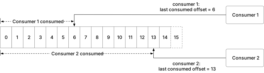
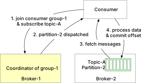
Consumer rebalancing
Rebalancing occurs when: consumer joins, leaves, crashes, or partitions change.
**Coordinator (Figure 16):** One broker per consumer group, found by hashing group name. Maintains consumer list, receives heartbeats, manages offsets. When list changes → elects new group leader → leader generates partition plan → coordinator broadcasts.
**Scenarios:** - Figure 17: General rebalance flow. - Figure 18: New consumer B joins → coordinator notifies A to rejoin → leader elected → partition plan generated and broadcast. - Figure 19: Consumer A leaves gracefully → coordinator rebalances remaining consumers. - Figure 20: Consumer A crashes → coordinator detects missing heartbeat → marks dead → triggers rebalance.
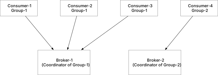
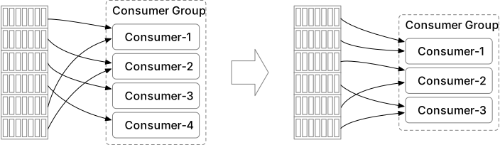
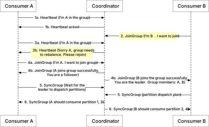
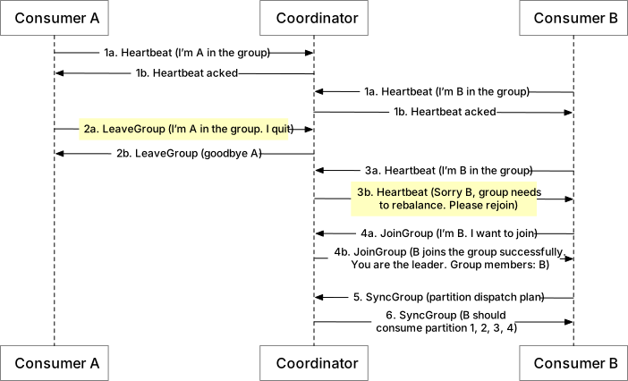
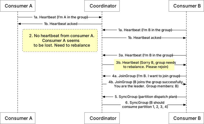
State storage
Stores: partition-to-consumer mapping, last consumed offsets per consumer group per partition (Figure 21).
Access patterns: frequent read/write, data updated frequently, random access, consistency important.
Recommendation: KV store like Zookeeper. Kafka moved offset storage from Zookeeper to Kafka brokers themselves.
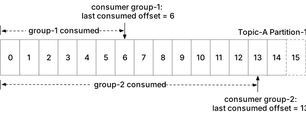
Metadata storage and ZooKeeper
Metadata storage: topic configuration (partitions, retention, replica distribution). Low volume, infrequent changes, high consistency → Zookeeper.
**ZooKeeper simplified design (Figure 22):** - Metadata + state storage moved to Zookeeper. - Broker only maintains data storage for messages. - Zookeeper handles broker leader election.
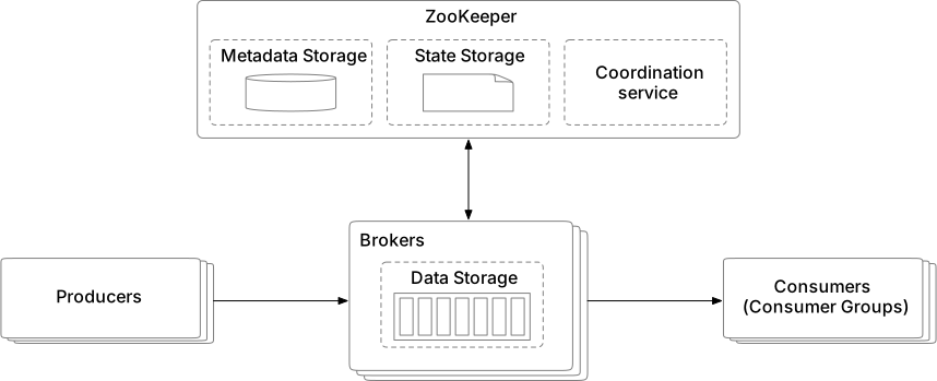
Replication
Each partition has 3 replicas across different brokers (Figure 23). One replica is leader, others are followers. Producers send to leader only. Followers pull from leader.
Replica distribution plan: elected broker controller generates the plan and stores in metadata.
**In-sync replicas (ISR) (Figure 24):** ISR = replicas within `replica.lag.max.messages` of the leader. Leader tracks ISR list by computing lag. - Replica-2, Replica-3: fully synced → in ISR. - Replica-4: lagged beyond threshold → removed from ISR until it catches up.
**ACK settings:** - ACK=all (Figure 25): ACK after ALL ISRs receive message → strongest durability, highest latency. - ACK=1 (Figure 26): ACK after leader persists → improved latency, risk of data loss if leader fails before replication. - ACK=0 (Figure 27): No ACK, no retry → lowest latency, acceptable data loss (metrics, logging).
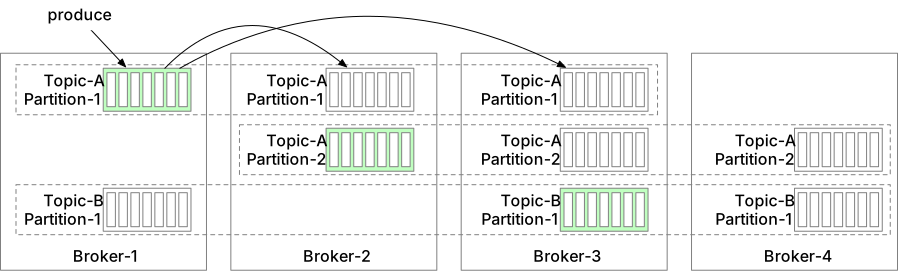
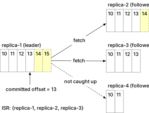
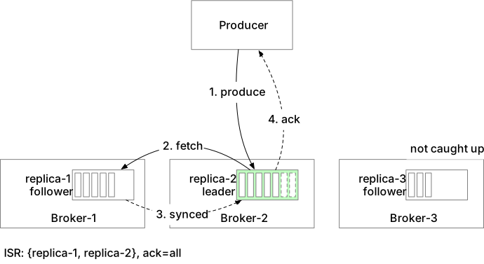
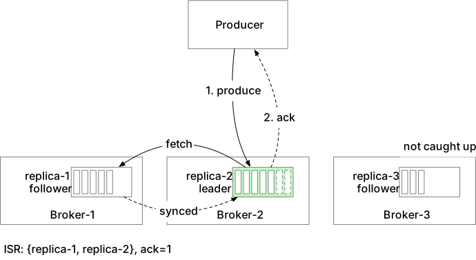
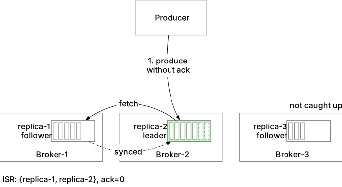
Scalability
**Producer:** Stateless — add/remove instances freely.
**Consumer:** Consumer groups isolated → add/remove groups freely. Rebalancing handles consumer changes within groups.
**Broker failure and recovery (Figure 28):** Broker 3 crashes → controller detects via coordination service → generates new replica distribution plan → new replicas in remaining brokers catch up from leaders.
**Adding broker (Figure 29):** Controller temporarily allows extra replicas → new broker catches up → redundant replica on old broker gracefully removed. No data loss.
**Partition increase (Figure 30):** Existing messages stay in old partitions (no migration). New messages distributed across all partitions. Producer/consumer notified automatically.
**Partition decrease (Figure 31):** Decommissioned partition stops receiving new messages but remains readable until retention period expires. Space freed only after retention period.
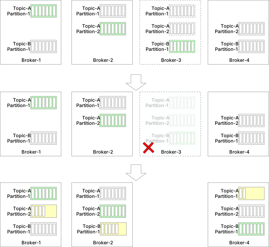
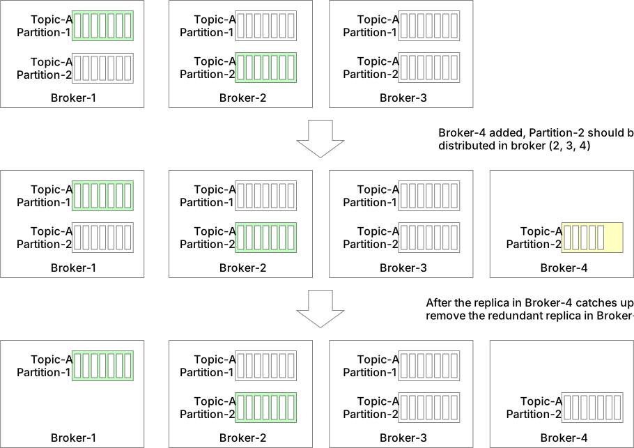
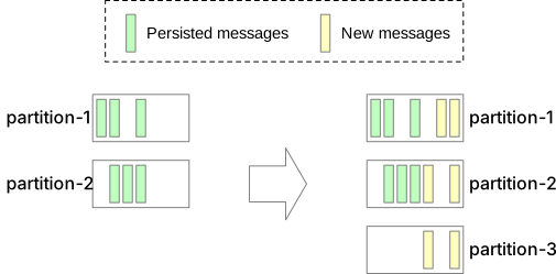
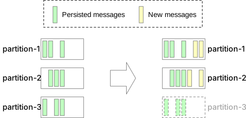
Data delivery semantics
**At-most once (Figure 32):** - Producer: ACK=0, no retry. - Consumer: commits offset BEFORE processing. - Messages may be lost but never redelivered. Use case: monitoring metrics.
**At-least once (Figure 33):** - Producer: ACK=1 or ACK=all, retries on failure. - Consumer: commits offset only AFTER successful processing. - Messages never lost but may be duplicated. Use case: most general cases (dedup by unique key in consumer).
**Exactly once (Figure 34):** - Hardest to implement; highest cost. - Use case: financial transactions (payment, trading, accounting) where duplication is unacceptable.



Advanced features
**Message filtering (Figure 35):** Consumer groups may want only subtypes of a topic's messages. Naive: consumer fetches all and filters locally (wastes bandwidth). Better: attach tags to messages, filter on broker side without accessing payload. Consumer subscribes by tag.
**Delayed/scheduled messages (Figure 36):** Delayed messages sent to temporary storage on broker, delivered to topic after delay expires. Core components: temporary storage (special topics) + timing function (delay queues with predefined levels, or hierarchical time wheel).
Use case: 30-minute payment timeout — send delayed message immediately, deliver to consumer 30 min later to check payment status.

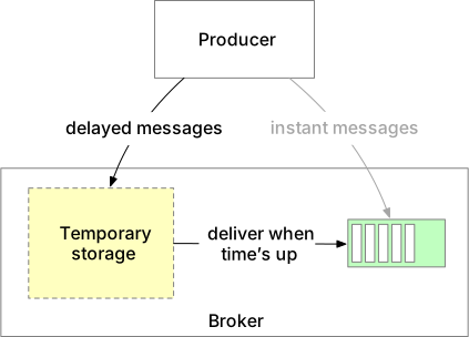
Step 4 - Wrap Up
Key design choices: WAL on-disk storage, no-copy message transit, pervasive batching, ISR-based replication, configurable ACK.
**Additional topics:** - Protocol: AMQP or Kafka protocol — covers production/consumption/heartbeat, efficient data transport, integrity verification. - Retry consumption: failed messages → dedicated retry topic for later reprocessing. - Historical data archive: HDFS or object storage for replaying truncated historical messages.
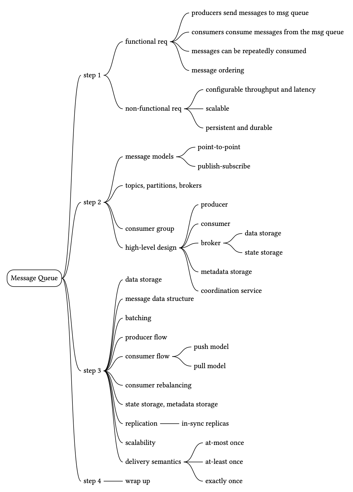
Metrics Monitoring and Alerting System
We design a scalable metrics monitoring and alerting system for internal use by a large company (similar to Datadog, Splunk). Figure 1 shows popular services in this space. A well-designed system provides clear visibility into infrastructure health, ensuring high availability and reliability.
Step 1 - Understand the Problem and Establish Design Scope
**Requirements:** - Internal system for large company. - Collect operational system metrics (CPU load, memory, disk, requests/sec, message queue counts). No log monitoring, no distributed tracing. - Scale: 100M DAU, 1,000 server pools × 100 machines × 100 metrics = **~10 million metrics**. - 1-year retention with downsampling: - 0-7 days: raw form. - 7-30 days: 1-minute resolution. - 30 days-1 year: 1-hour resolution. - Alert channels: email, phone, PagerDuty, webhooks.
**Non-functional requirements:** - Scalable (growing metrics and alert volume). - Low latency (dashboards and alerts). - Highly reliable (no missing critical alerts). - Flexible pipeline (easy technology integration).
Step 2 - Propose High-Level Design and Get Buy-In
Fundamentals
Five components of a metrics monitoring system (Figure 2): 1. **Data collection:** collect metric data from sources. 2. **Data transmission:** transfer data to the monitoring system. 3. **Data storage:** organize and store incoming data. 4. **Alerting:** analyze data, detect anomalies, send alerts to channels. 5. **Visualization:** display data in graphs and charts.
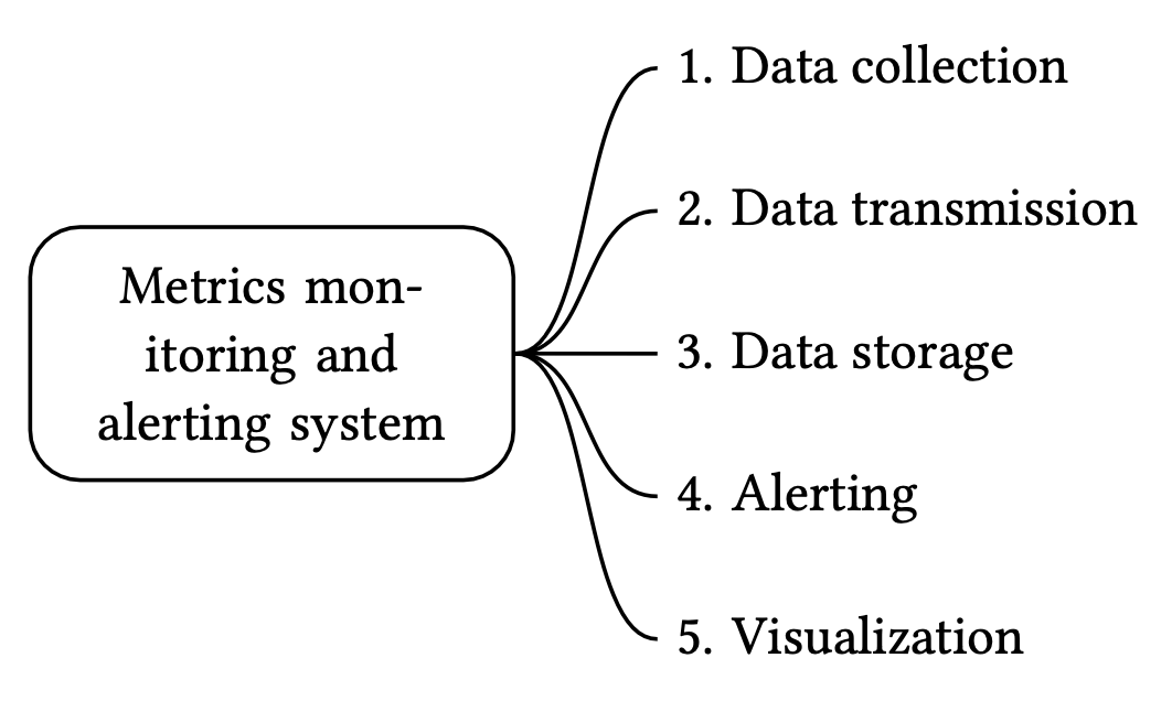
Data model
Metrics data is a time series: a set of values with associated timestamps, uniquely identified by metric name + labels.
**Example (Figure 3):** CPU load on server i631 at 20:00 → `{metric_name: cpu.load, labels: host:i631,env:prod, timestamp: 1613707265, value: 0.29}`
**Line protocol format:** `CPU.load host=webserver01,region=us-west 1613707265 50`
Time series schema: - Metric name (string) - Labels/tags (list of key:value pairs) - Array of (value, timestamp) pairs
**Data access pattern (Figure 4):** - **Write:** heavy — ~10M metrics written constantly at high frequency. - **Read:** spiky — visualization and alerting cause bursty reads.
**Data storage — why time-series DB:** - General-purpose DB (MySQL): poor fit — complex SQL for time-window queries, requires per-tag indexes, struggles under constant heavy writes. - NoSQL (Cassandra, Bigtable): possible but requires deep expertise for scalable time-series schema. - **Time-series DB (InfluxDB, Prometheus):** optimized for sequential writes, custom query languages, built-in label indexing, data retention/aggregation features.
Figure 5: InfluxDB with 8 cores + 32 GB RAM handles **250,000+ writes/sec**.


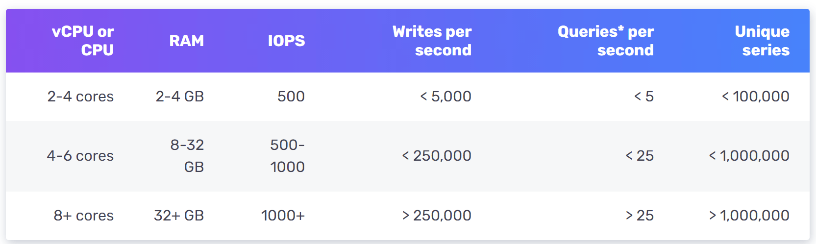
High-level design
Figure 6 shows the high-level design components: - **Metrics source:** application servers, DBs, message queues. - **Metrics collector:** gathers metrics, writes to time-series DB. - **Time-series database:** stores metrics with custom query interface + label indexes. - **Query service:** thin wrapper over time-series DB for visualization and alerting systems. - **Alerting system:** sends notifications to channels. - **Visualization system:** graphs and charts for engineers.
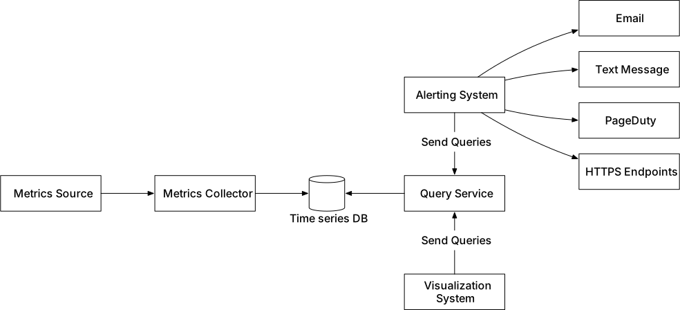
Step 3 - Design Deep Dive
Metrics collection
Occasional data loss is acceptable (fire and forget). Figure 7 shows the metrics collection flow.
**Pull model (Figure 8):** Dedicated metrics collectors pull metrics from running applications over HTTP (e.g., `/metrics` endpoint).
**Service discovery (Figure 9):** Collectors use etcd/Zookeeper to discover service endpoints. Configuration includes: pulling interval, IP addresses, timeout, retry parameters.
**Pull model in detail (Figure 10):** 1. Collector fetches endpoint config from Service Discovery. 2. Pulls metrics via HTTP `/metrics` endpoint (client library required). 3. Optionally registers for change events from Service Discovery.
**Scaling pull model (Figure 11):** Use consistent hashing ring with multiple collectors. Each collector owns a range of the ring → each source server assigned to exactly one collector (no duplicates).
**Push model (Figure 12):** Collection agents installed on each server push metrics periodically to collectors. Agent can aggregate locally before sending. Auto-scaling collector cluster with load balancer (Figure 13) prevents overload.
**Pull vs push comparison:**
| | Pull | Push | |---|---|---| | Debugging | Easy — `/metrics` accessible anytime | Harder | | Health check | Easy — no response = server down | Hard to distinguish network issue from no data | | Short-lived jobs | Misses them (fix: push gateways) | Wins | | Network setup | All endpoints must be reachable | Load balancer can receive from anywhere | | Protocol | TCP | UDP (lower latency) | | Data authenticity | Defined in config files | Any client can push (fix: whitelist/auth) |
Examples: Pull → Prometheus. Push → Amazon CloudWatch, Graphite.
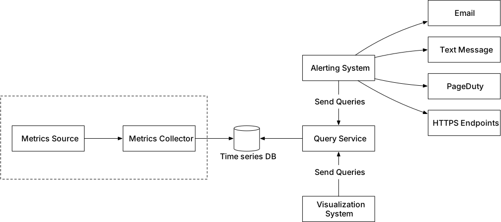
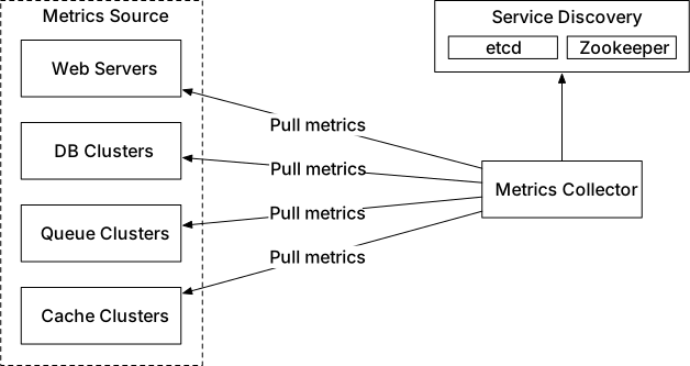
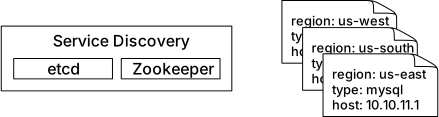
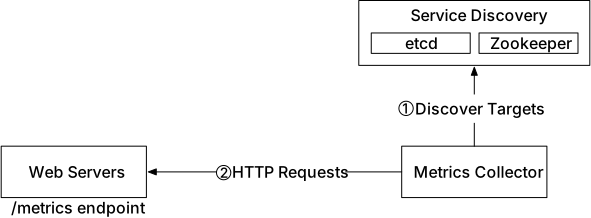
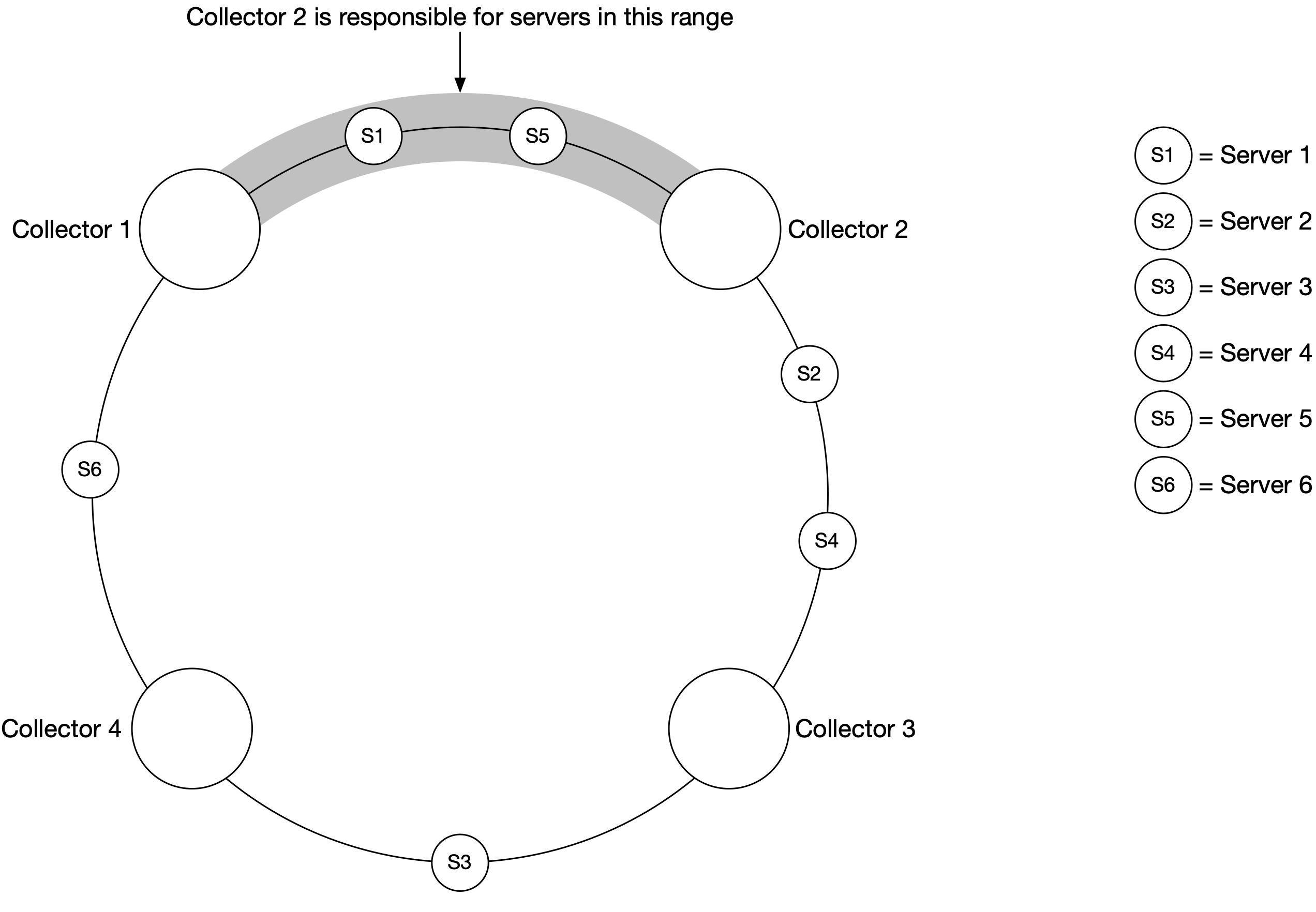
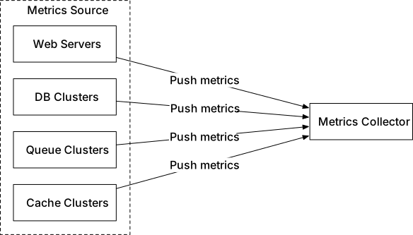
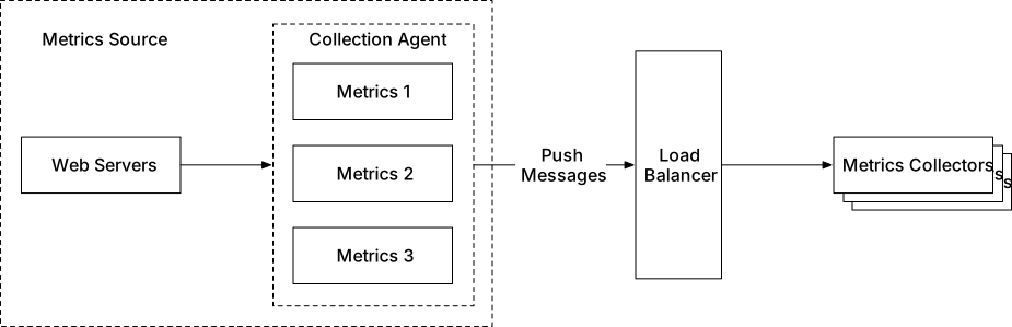
Scale the metrics transmission pipeline
Metrics collector cluster receives enormous data from either model (Figure 14). Risk: data loss if time-series DB is unavailable.
**Solution (Figure 15):** Add Kafka as queue between collectors and time-series DB. Stream processors (Apache Storm, Flink, Spark) consume from Kafka and write to TSDB.
Benefits: - Highly reliable and scalable messaging platform. - Decouples data collection from processing. - Prevents data loss when DB is unavailable.
**Scale through Kafka (Figure 16):** - Configure partition count based on throughput. - Partition by metric name → consumers aggregate by metric. - Further partition by tags/labels. - Prioritize important metrics.
**Alternative to Kafka:** Facebook's Gorilla in-memory time-series DB avoids intermediate queue by designing for high write availability even during partial network failures.
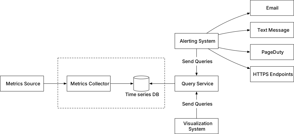
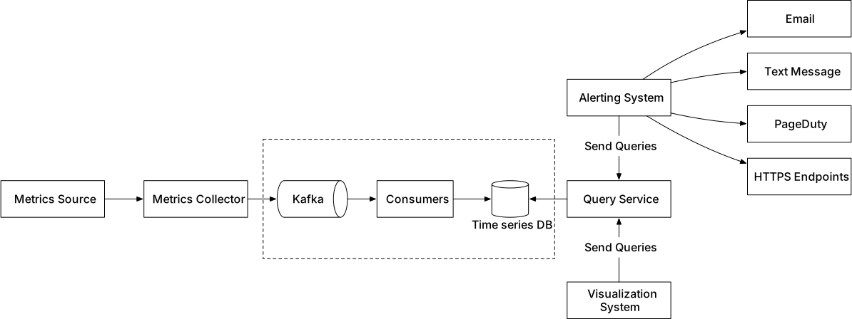
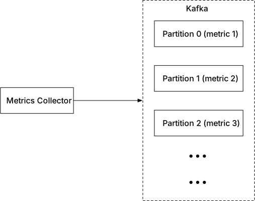
Query service
Cluster of query servers accessing time-series DB for visualization/alerting clients. Decouples TSDB from clients — flexibility to swap either.
**Cache layer (Figure 17):** Cache servers store query results to reduce TSDB load.
**Time-series query language:** Prometheus and InfluxDB use custom languages (PromQL, Flux) instead of SQL. Reason: complex SQL for time-window analysis.
SQL for exponential moving average (complex): ```sql select id, temp, avg(temp) over (partition by group_nr order by time_read) ... ```
Flux (simple): ``` from(db:"telegraf") |> range(start:-1h) |> filter(...) |> exponentialMovingAverage(size:-10s) ```
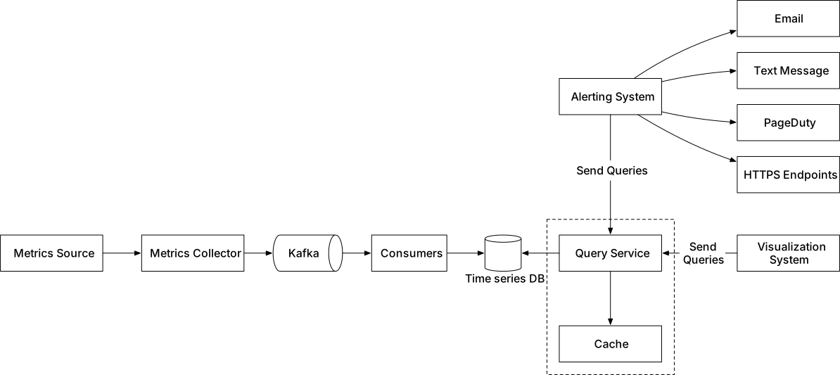
Storage layer
**Data encoding and compression (Figure 18):** 85% of queries are for data collected in past 26 hours (Facebook research). Use delta encoding: store 1610087371, 10, 10, 9, 11 instead of full timestamps → 4 bits vs 32 bits per delta.
**Downsampling:** Convert high-resolution → low-resolution to reduce disk usage. - 0-7 days: no sampling (raw). - 7-30 days: 1-minute resolution. - 30 days-1 year: 1-hour resolution.
Example: 10-second data → 30-second data by averaging three data points.
**Cold storage:** Inactive/old data moved to cold storage (much lower cost).
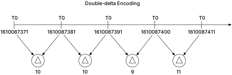
Alerting system
Figure 19 shows the alerting system flow:
1. **Load alert config to cache:** Rules defined in YAML files. ```yaml - name: instance_down rules: - alert: instance_down expr: up == 0 for: 5m labels: severity: page ``` 2. **Alert manager fetches config** from cache. 3. **Alert manager calls query service** at predefined intervals. If threshold violated → alert event created. Responsibilities: - **Filter, merge, dedupe (Figure 20):** Merge multiple alerts for same instance within short time window. - **Access control:** Restrict operations to authorized users. - **Retry:** Ensure at least once notification delivery. 4. **Alert store:** KV database (Cassandra) storing alert state (inactive → pending → firing → resolved). 5. Eligible alerts → Kafka. 6. Alert consumers pull from Kafka. 7. Alert consumers send notifications via email, SMS, PagerDuty, HTTP webhooks.
**Build vs buy:** Industrial-scale alerting systems (e.g., Grafana Alerting) integrate with popular TSDB and notification channels. Strong case for buying.
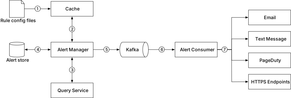
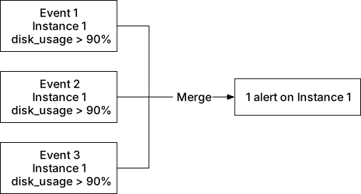
Visualization system
Built on top of the data layer. Figure 21 shows Grafana UI displaying server requests, memory/CPU utilization, page load time, traffic, login info.
Recommendation: Use Grafana (off-the-shelf). Hard to build high-quality visualization system; Grafana integrates well with popular time-series databases.
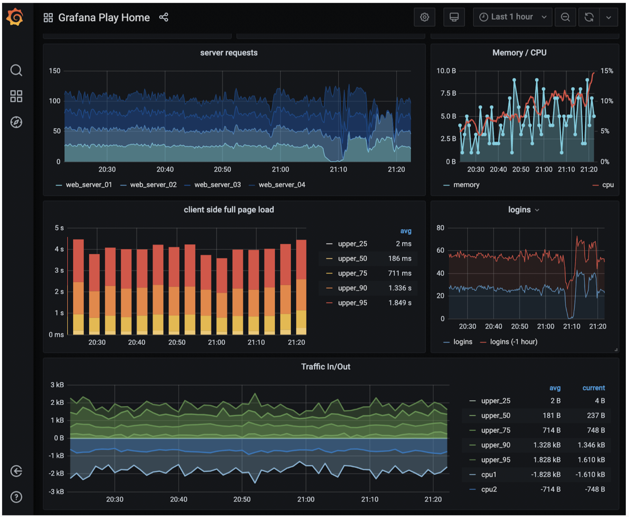
Step 4 - Wrap Up
Key design topics: pull vs push collection, Kafka for scale, time-series DB selection, downsampling for storage optimization, build vs buy for alerting/visualization.
Figure 22 shows the final integrated design.
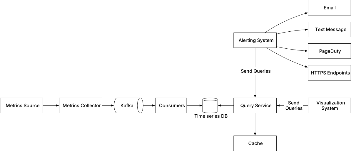
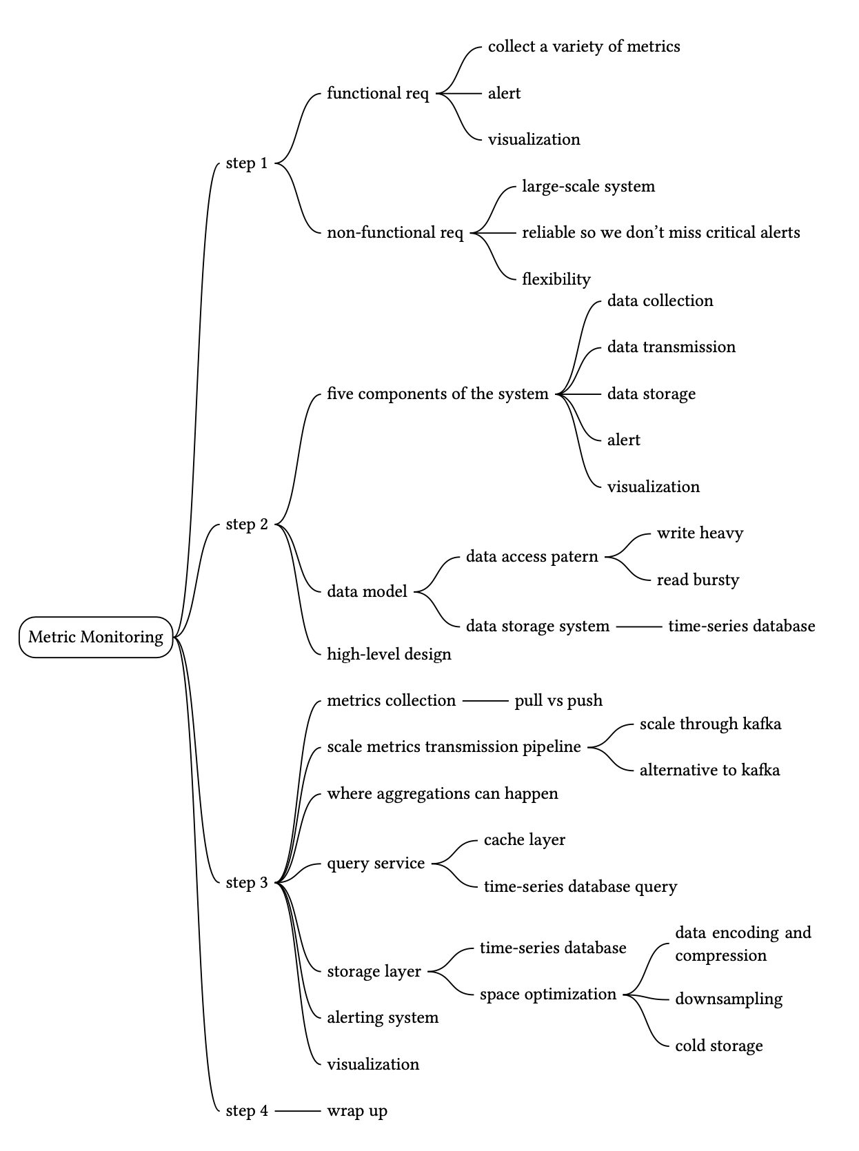
Ad Click Event Aggregation
We design an ad click event aggregation system at Facebook/Google scale. Digital advertising uses Real-Time Bidding (RTB) — inventory bought and sold in under one second (Figure 1). Key metrics like CTR (click-through rate) and CVR (conversion rate) depend on aggregated click data. Data accuracy is critical as it directly impacts advertiser billing.

Step 1 - Understand the Problem and Establish Design Scope
**Functional requirements:** - Input: log files with `ad_id, click_timestamp, user_id, ip, country`. - Query 1: number of click events for a given ad_id in last M minutes. - Query 2: top 100 most clicked ads in past 1 minute (configurable). - Query 3: filter by ip, user_id, or country. - Handle late-arriving events, duplicated events, and system recovery.
**Non-functional requirements:** - Correctness (used for RTB and billing). - Proper handling of delayed and duplicate events. - Robustness (resilient to partial failures). - End-to-end latency: a few minutes at most.
**Back-of-the-envelope estimation:** - 1 billion ad click events/day. - Avg QPS = 10^9 / 10^5 = **10,000 QPS**; peak QPS = **50,000**. - Storage: 0.1 KB × 1B = **100 GB/day** (~3 TB/month).
Step 2 - Propose High-Level Design and Get Buy-In
Query API design
**API 1:** Aggregate click count for an ad. ``` GET /v1/ads/{:ad_id}/aggregated_count Params: from (start minute), to (end minute), filter (filtering strategy id) Response: { ad_id, count } ```
**API 2:** Top N clicked ads. ``` GET /v1/ads/popular_ads Params: count (top N), window (M minutes), filter (filtering strategy id) Response: { ad_ids: [...] } ```
Data model
**Raw data (log files):** ``` [AdClickEvent] ad001, 2021-01-01 00:00:01, user1, 207.148.22.22, USA ``` Fields: `ad_id, click_timestamp, user_id, ip, country`
**Aggregated data (per minute):** `ad_id, click_minute, count` — optionally with `filter_id` for filtering support.
**Top N data:** `window_size, update_time_minute, most_clicked_ads (JSON array)`
**Recommendation: store BOTH raw and aggregated data.** - Raw data: backup for recalculation, debugging. Moved to cold storage when old. - Aggregated data: active data optimized for query performance.
**Database selection:** Write-heavy (10K avg QPS). NoSQL like Cassandra or InfluxDB preferred for both raw and aggregated data (optimized for write + time-range queries). Alternative: store raw data in S3 using columnar formats (ORC, Parquet, AVRO).
High-level design
Figure 2 shows the aggregation workflow. Figure 3 shows the full high-level design with two Kafka queues:
- **Kafka 1:** raw ad click events. - **Aggregation service:** MapReduce processing. - **Kafka 2:** aggregated results (click counts per minute + top N ads per minute). - **Database writer:** polls Kafka 2, writes to DB.
Reason for Kafka 2 (not writing directly to DB): needed for end-to-end exactly-once semantics via atomic commit (Figure 4).
**Aggregation service — MapReduce DAG (Figure 5):** - **Map node (Figure 6):** reads from data source, filters and routes events. E.g., ads with `ad_id % 2 = 0` → node 1, others → node 2. - **Aggregate node:** counts ad click events by ad_id in memory every minute (in-memory counting). - **Reduce node (Figure 7):** reduces aggregated results from all Aggregate nodes to final result.
Intermediate data stored in memory; nodes communicate via TCP (different processes) or shared memory (same process).
**Use cases:** - Figure 8: count clicks — input partitioned by `ad_id % 3` → each Aggregate node counts independently. - Figure 9: top N ads — each Aggregate node maintains a heap for top 3 ads → Reduce node merges to final top N. - Filtering: star schema — pre-aggregate by dimension (country, ip, user_id). Records have `ad_id, click_minute, country, count`.

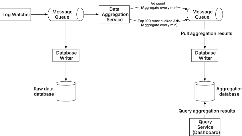
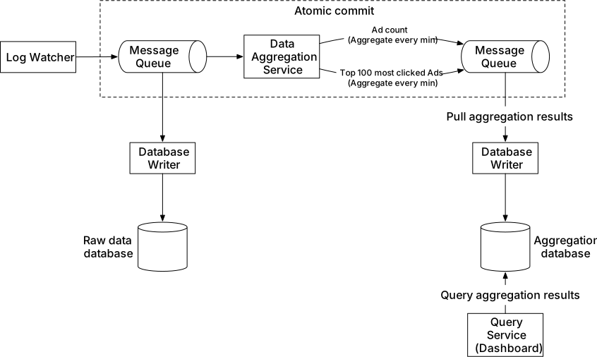
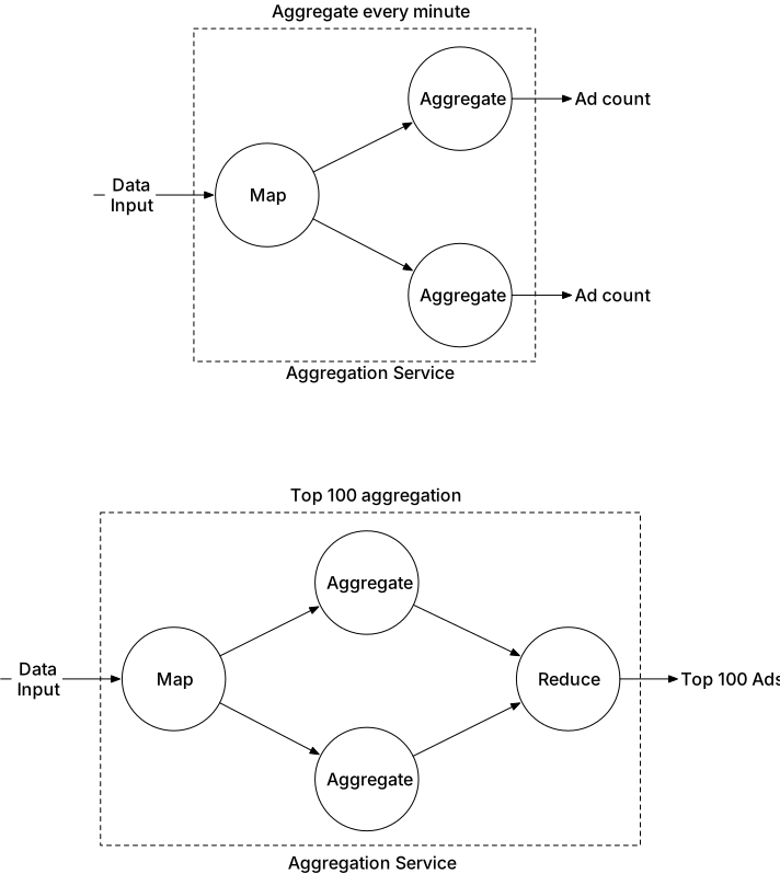
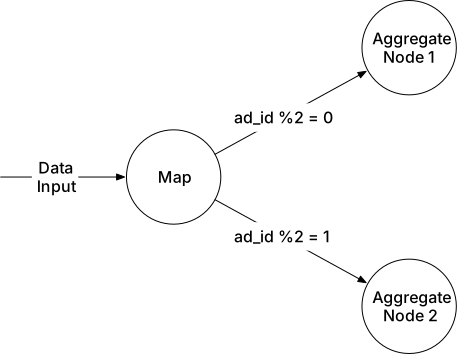
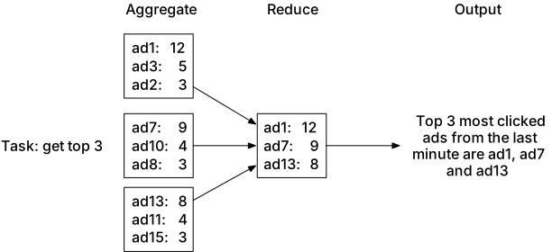
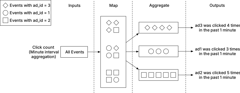
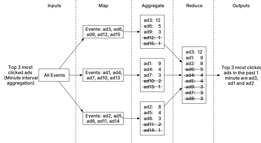
Step 3 - Design Deep Dive
Streaming vs batching
Our design uses both stream processing (real-time aggregation) and batch processing (historical data backup).
**Lambda architecture:** Two processing paths (batch + streaming) simultaneously. Disadvantage: two codebases to maintain.
**Kappa architecture (our choice, Figure 10):** Single stream processing path for both real-time and historical reprocessing. Simpler — one codebase.
**Data recalculation (Figure 11):** When a bug is found in the aggregation service: 1. Recalculation service retrieves raw data from cold storage (batch job). 2. Sends to a dedicated aggregation service (separate from real-time, so no impact). 3. Aggregated results → Kafka 2 → DB update.
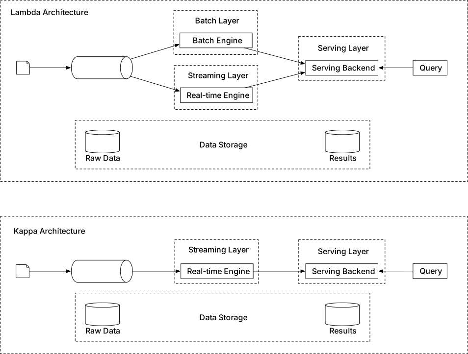
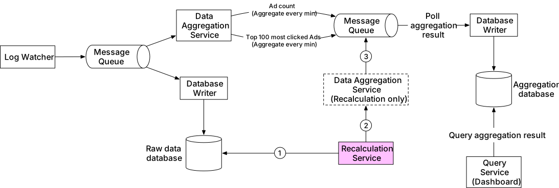
Time and aggregation window
**Event time vs processing time (Figure 12):** - Event time: when ad is clicked → more accurate, but depends on client clock (can be wrong/malicious). - Processing time: server system time → more reliable, but inaccurate for late-arriving events. - Recommendation: **event time** for accuracy.
**Watermark technique (Figures 13, 14):** Extends aggregation window by configurable duration (e.g., 15 seconds) to catch slightly late events. - Long watermark: better accuracy, higher latency. - Short watermark: lower latency, some data loss. - Very late events: handle via end-of-day reconciliation.
**Tumbling window (Figure 15):** Fixed non-overlapping time chunks. Best for use case 1 (count per minute).
**Sliding window (Figure 16):** Overlapping window that slides with configured interval. Best for use case 2 (top N in last M minutes).
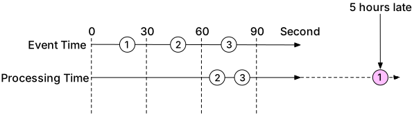
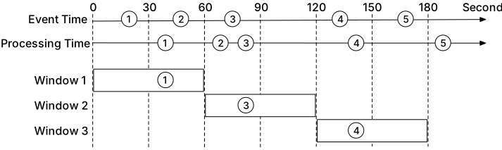
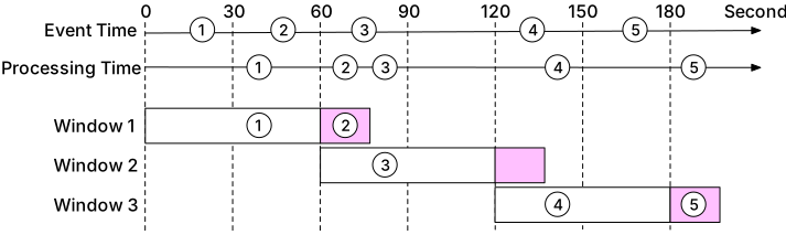
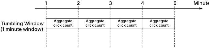
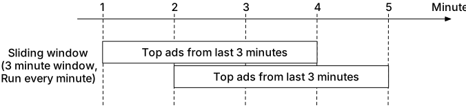
Delivery guarantees
Since aggregation is used for billing, **exactly-once** delivery is required (not at-least-once). A few percent discrepancy = millions of dollars in billing errors.
**Data deduplication — duplicate sources:** 1. Client-side: malicious resending → handled by ad fraud/risk control components. 2. Server outage (Figure 17): Aggregator crashes after sending to downstream but before committing offset → next Aggregator re-processes same events.
**Offset tracking solutions:** - Figure 18: Store offset in external storage (HDFS/S3) BEFORE sending downstream. Problem: if downstream send fails, offset already written → events lost. - Figure 19: Store offset AFTER getting ACK from downstream. Problem: if Aggregator crashes before saving offset → events processed again (duplicate). - Figure 20: Wrap steps 4-6 in a **distributed transaction** → exactly-once guarantee. If any step fails, entire transaction rolls back.
Exactly-once in large-scale systems is complex — refer to Apache Flink's end-to-end exactly-once for details.


Scale the system
Business grows 30%/year → doubles every 3 years. Scale each component independently.
**Scale message queue:** - Producers: no limit on instances. - Consumers (Figure 21): add consumers in group → rebalancing distributes partitions. Do this during off-peak hours (rebalance can take minutes). - Brokers: use `ad_id` as Kafka hashing key → same ad events go to same partition. Pre-allocate enough partitions. Shard topics by geography or business type.
**Scale aggregation service (Figure 22):** - Option 1: Multi-threading — different `ad_id` ranges to different threads (Figure 23). Easier to implement. - Option 2: Multi-processing via YARN — horizontally scalable. More widely used in production.
**Scale database:** Cassandra natively supports horizontal scaling with consistent hashing (Figure 24 — virtual nodes). Adding a node automatically rebalances — no manual resharding.
**Hotspot issue (Figure 25):** Popular ads (large advertisers) receive disproportionate events. - Aggregation node detects overload → requests more resources from resource manager. - Resource manager allocates additional nodes → original node splits events across nodes → results aggregated back. - Advanced: Global-Local Aggregation or Split Distinct Aggregation.
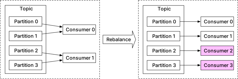
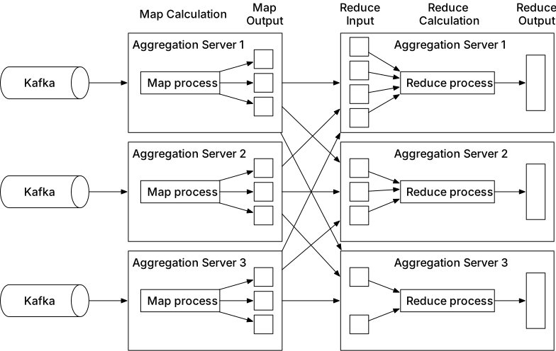
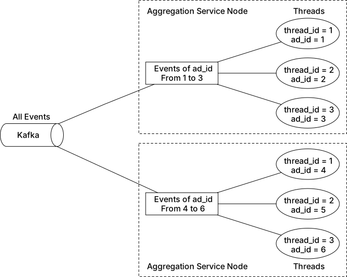
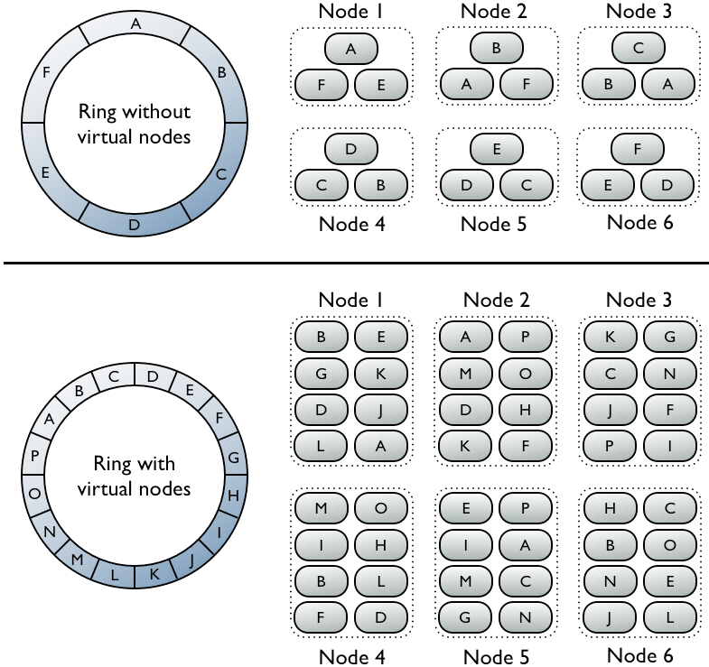
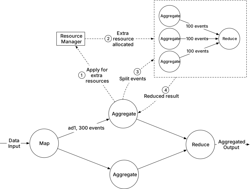
Fault tolerance
Aggregation happens in-memory → node failure loses in-memory state.
**Snapshot mechanism (Figure 26):** Periodically save system status (upstream Kafka offset + top-N aggregation state) to a snapshot.
**Failover (Figure 27):** New node starts from latest snapshot, replays only events after the snapshot from Kafka broker. Fast recovery — no need to replay from beginning.
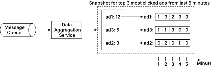
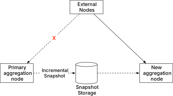
Step 4 - Wrap Up
Key design topics: MapReduce DAG for aggregation, Kappa architecture for unified batch+streaming, watermark for late events, distributed transactions for exactly-once, snapshot-based fault tolerance.
Figure 28 shows the final design with reconciliation support. Figure 29 shows an alternative design using Hive + ElasticSearch + ClickHouse/Druid for OLAP-based aggregation.
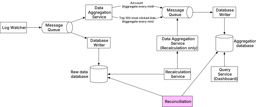
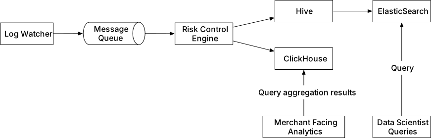
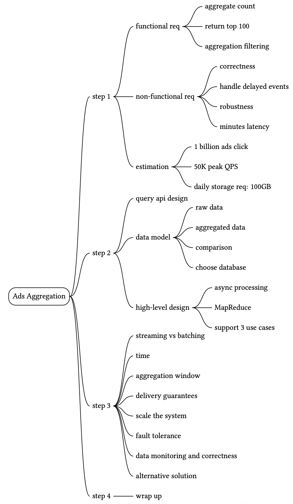
Hotel Reservation System
We design a hotel reservation system for a hotel chain such as Marriott International. The design and techniques are also applicable to other booking-related interview topics: Design Airbnb, Design a flight reservation system, Design a movie ticket booking system.
Step 1 - Understand the Problem and Establish Design Scope
**Functional requirements:** - Hotel chain with **5,000 hotels and 1 million rooms** in total. - Customers pay in full when they make reservations. - Booking via hotel website or app only. - Customers can cancel reservations. - **10% overbooking** supported (hotels sell more rooms than capacity to anticipate cancellations). - Scope: hotel detail page, room detail page, room reservation, admin panel, overbooking. - Room prices change dynamically (depends on expected occupancy for a given day).
**Non-functional requirements:** - Support high concurrency — popular hotels may have many users booking the same room during peak season. - Moderate latency — a few seconds to process a reservation is acceptable.
**Back-of-the-envelope estimation (Figure 1):** - 5,000 hotels, 1M rooms, 70% occupancy, 3-day average stay. - Daily reservations: (1M × 0.7) / 3 ≈ **240,000/day**. - Reservation TPS: 240,000 / 10⁵ seconds ≈ **3 TPS**. - Typical customer funnel (10% conversion at each step): - Hotel detail page QPS: **300** - Booking page QPS: **30** - Final reservation TPS: **3**
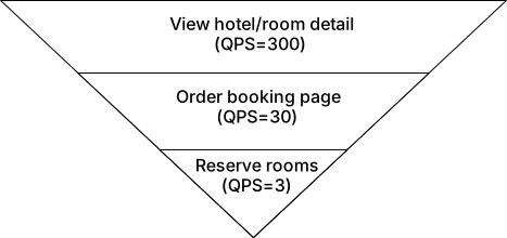
Step 2 - Propose High-Level Design and Get Buy-In
API design
RESTful APIs for hotel, room, and reservation management.
**Hotel APIs:** | API | Detail | |-----|--------| | GET /v1/hotels/ID | Get hotel details | | POST /v1/hotels | Add hotel (staff only) | | PUT /v1/hotels/ID | Update hotel (staff only) | | DELETE /v1/hotels/ID | Delete hotel (staff only) |
**Room APIs:** | API | Detail | |-----|--------| | GET /v1/hotels/ID/rooms/ID | Get room details | | POST /v1/hotels/ID/rooms | Add room (staff only) | | PUT /v1/hotels/ID/rooms/ID | Update room (staff only) | | DELETE /v1/hotels/ID/rooms/ID | Delete room (staff only) |
**Reservation APIs:** | API | Detail | |-----|--------| | GET /v1/reservations | Get reservation history | | GET /v1/reservations/ID | Get reservation details | | POST /v1/reservations | Make new reservation | | DELETE /v1/reservations/ID | Cancel reservation |
**Make reservation request body:** ```json { "startDate": "2021-04-28", "endDate": "2021-04-30", "hotelID": "245", "roomID": "U12354673389", "reservationID": "13422445" } ```
`reservationID` is the **idempotency key** to prevent double booking.
Data model
Access patterns: 1. View detailed information about a hotel. 2. Find available types of rooms given a date range. 3. Record a reservation. 4. Look up a reservation or past history.
**Why relational database:** - Read-heavy, write-less workflow (users browsing >> users booking). - ACID guarantees — critical for preventing double bookings, negative balances, double charges. - Clear, stable data model with well-defined relationships (hotel, room, room_type).
**Initial schema (Figure 2):** hotel → room → reservation tables. The `status` field in reservation table follows the state machine shown in Figure 3 (pending → paid/canceled → refunded/rejected).
**Important limitation:** This schema ties reservations to specific rooms (room_id). However, in hotels, customers reserve a *type* of room, not a specific room. Room numbers are assigned at check-in. This is addressed in the improved data model (deep dive).
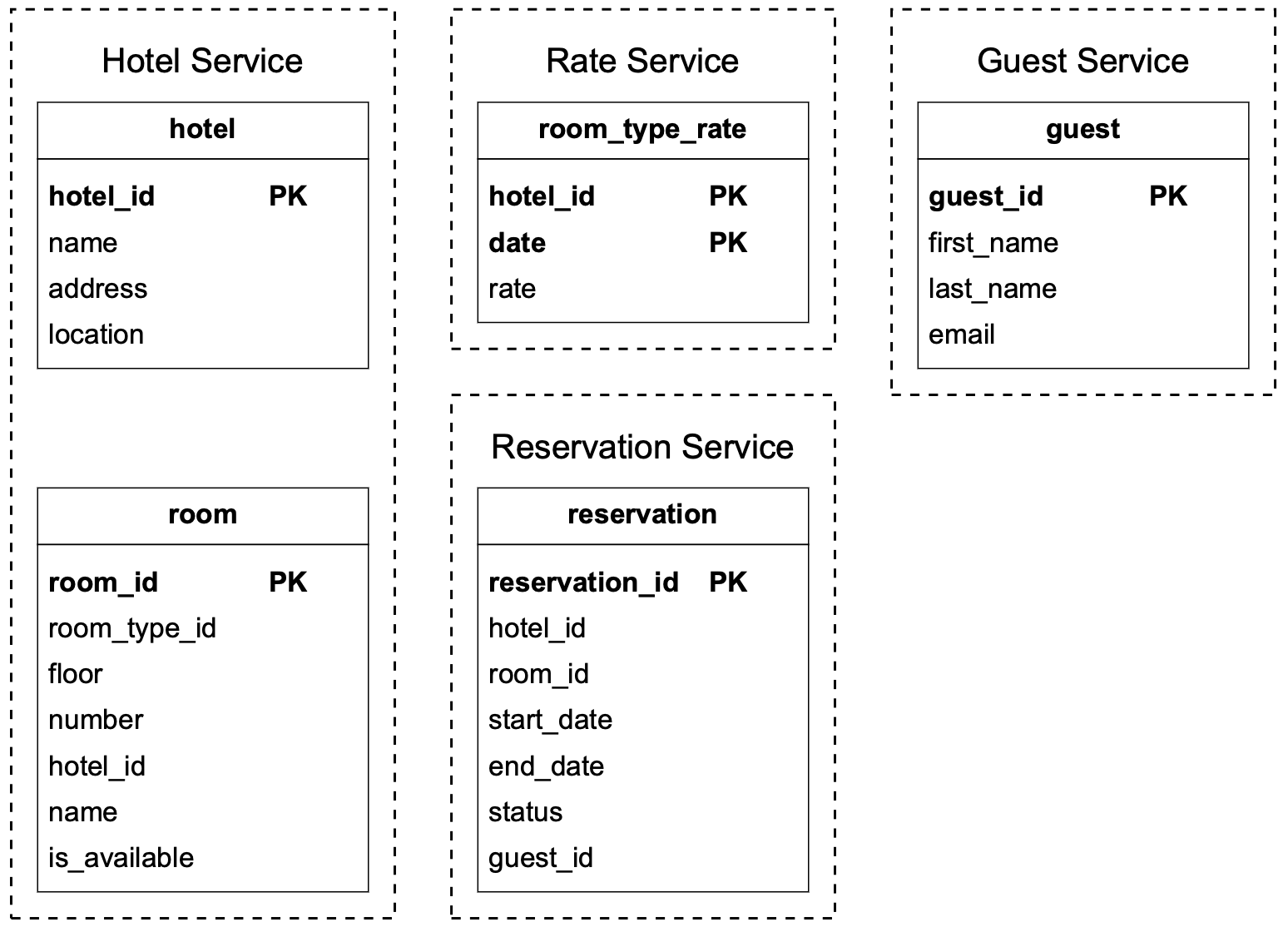
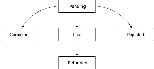
High-level design
Microservice architecture (Figure 4):
- **User** — books rooms via mobile or computer. - **Admin (hotel staff)** — manages reservations, refunds, room info. - **CDN** — caches static assets (JS, images, HTML) for faster load times. - **Public API Gateway** — rate limiting, authentication, routes requests to services. - **Internal APIs** — only accessible to authorized staff, protected by VPN. - **Hotel Service** — hotel and room details (mostly static, easily cached). - **Rate Service** — room prices for future dates (dynamic pricing). - **Reservation Service** — handles reservation requests and tracks room inventory. - **Payment Service** — executes payments, updates reservation status (paid/rejected). - **Hotel Management Service** — staff operations: view upcoming reservations, reserve rooms, cancel reservations.
Figure 5 shows inter-service connections: Reservation Service queries Rate Service to compute total room charge; Hotel Management Service forwards requests to the services owning the data.
Inter-service communication typically uses gRPC for modern, high-performance RPC.
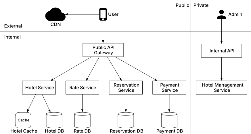
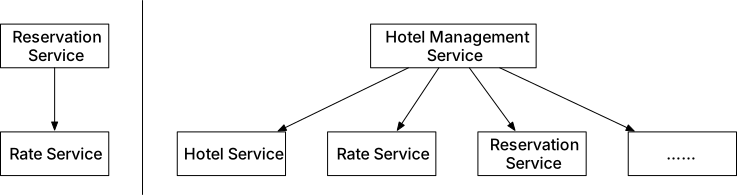
Step 3 - Design Deep Dive
Improved data model
**Key insight:** Customers reserve a *room type*, not a specific room. Updated reservation API uses `roomTypeID` + `roomCount` instead of `roomID`.
**Updated request:** ```json { "startDate": "2021-04-28", "endDate": "2021-04-30", "hotelID": "245", "roomTypeID": "12354673389", "roomCount": "3", "reservationID": "13422445" } ```
**Updated schema (Figure 6)** introduces the critical `room_type_inventory` table:
| Column | Description | |--------|-------------| | hotel_id | Hotel identifier | | room_type_id | Room type identifier | | date | Single date (one row per date) | | total_inventory | Total rooms minus rooms temporarily taken offline | | total_reserved | Total rooms booked for this hotel/type/date |
**Composite primary key:** (hotel_id, room_type_id, date)
Rows pre-populated for all future dates within 2 years; a daily job advances the window.
**Reservation check query:** ```sql SELECT date, total_inventory, total_reserved FROM room_type_inventory WHERE room_type_id = ${roomTypeId} AND hotel_id = ${hotelId} AND date BETWEEN ${startDate} AND ${endDate} ```
For each row: `if (total_reserved + numberOfRoomsToReserve) <= total_inventory` → room available.
**10% overbooking:** change condition to `<= 110% * total_inventory`.
**Storage estimate:** 5,000 hotels × 20 room types × 2 years × 365 days = **73 million rows** — fits in a single DB with replicas.
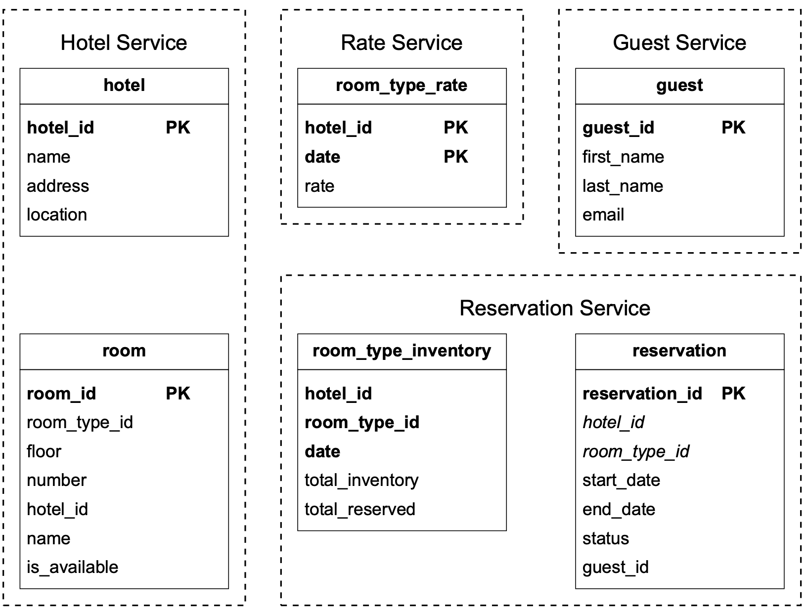
Concurrency issues
**Problem 1: Same user clicks "book" multiple times (Figure 7).**
Solutions: - **Client-side:** Gray out/disable submit button after click. Unreliable — users can bypass JavaScript. - **Idempotent API (Figure 8):** Include `reservationID` as idempotency key. Since `reservationID` is the primary key of the reservation table, the unique constraint prevents duplicate rows.
**Flow:** 1. Customer enters reservation details → clicks "Continue" → reservation order generated with a globally unique `reservationID`. 2. Confirmation page (Figure 9) shows order details including `reservationID`. 3. Customer clicks "Complete my booking" — `reservationID` sent as primary key. 4. If clicked twice, second insert violates primary key uniqueness → rejected (Figure 10).
**Problem 2: Multiple users book the same room when only 1 remains (Figure 11).**
Race condition: two transactions both read `total_reserved = 99` (1 room left), both pass the check, both commit → 101 reserved against 100 inventory.
Three locking strategies:
**Option 1: Pessimistic locking (Figure 12)** `SELECT ... FOR UPDATE` locks rows for the transaction's duration. - Pros: Prevents conflicts, simple to implement, effective under heavy contention. - Cons: Deadlock risk, not scalable (long-held locks block other transactions). - Verdict: **Not recommended** for this system.
**Option 2: Optimistic locking (Figure 13)** Adds a `version` column. Read version → update → write with `version + 1`. Database validation rejects writes where version doesn't match. - Pros: No DB locks, works well when contention is low. - Cons: Performance degrades under heavy contention — repeated retries degrade UX. - Verdict: **Good option** since hotel reservation QPS is typically low.
**Option 3: Database constraint (Figure 14)** ```sql CONSTRAINT check_room_count CHECK((total_inventory - total_reserved >= 0)) ``` Violation → transaction rollback. - Pros: Easy to implement, effective at low contention. - Cons: High contention causes many failures, constraints aren't easily version-controlled, not all DBs support them. - Verdict: **Good option** for low-QPS hotel reservations.
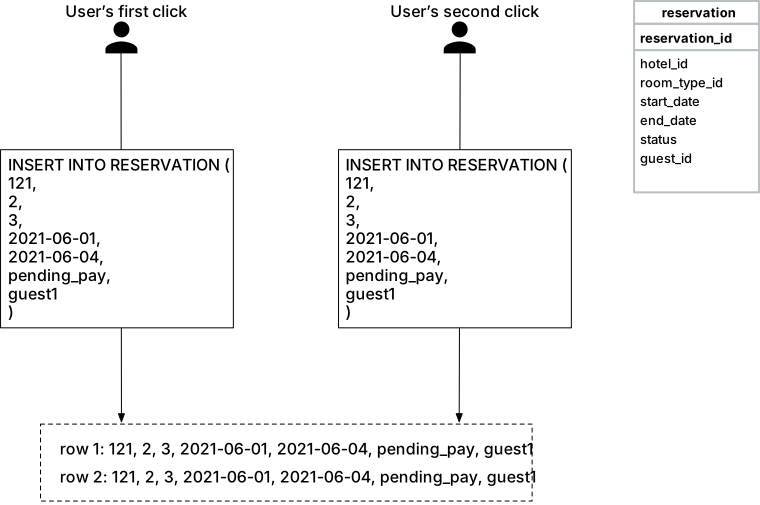
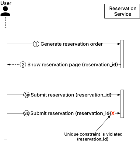

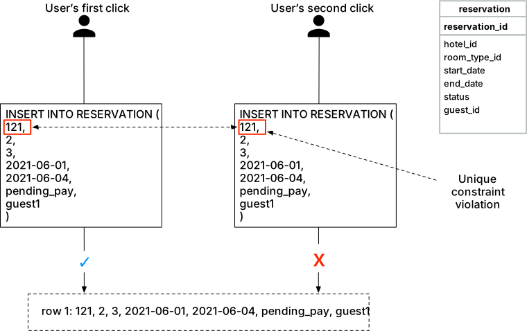
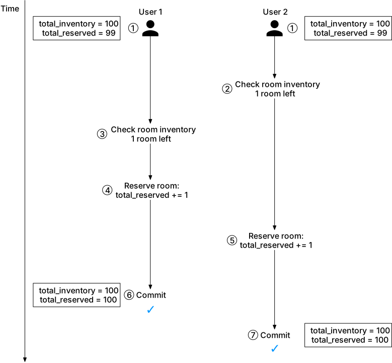
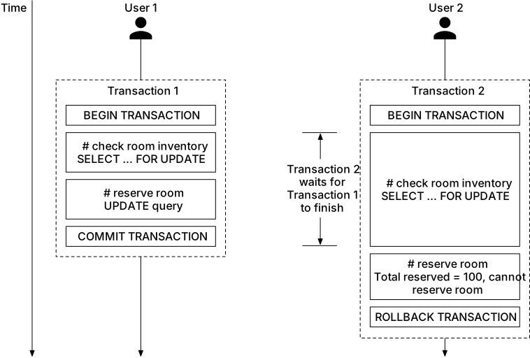
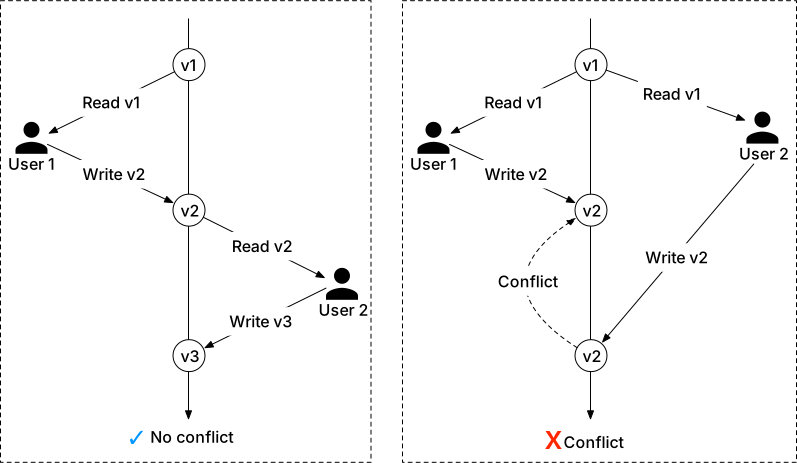
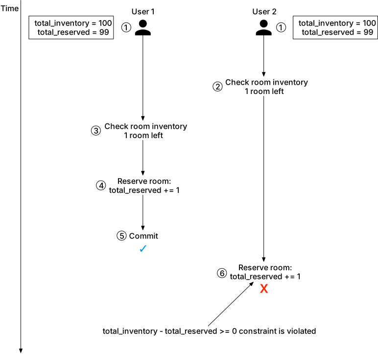
Scalability
For large-scale travel sites (booking.com, expedia.com), QPS could be 1,000× higher. All services are stateless and scale horizontally. Database is the bottleneck.
**Database sharding (Figure 15):** - Most queries filter by `hotel_id` → shard by `hotel_id`. - 16 shards: 30,000 QPS / 16 = **1,875 QPS per shard** (within MySQL capacity). - Shard key: `hash(hotel_id) % number_of_servers`.
**Caching (Figure 16):** - Hotel inventory is time-bounded — only current and future dates matter; old data is irrelevant. - Use **Redis** with TTL + LRU eviction for optimal memory use. - Move inventory check logic to cache: `key = hotelID_roomTypeID_{date}`, `value = available rooms`. - Read operations (check inventory) >> write operations (make reservation) → cache absorbs most reads.
**Cache consistency via CDC (Change Data Capture):** 1. DB updated first (source of truth). 2. Change propagated to Redis asynchronously via CDC (e.g., **Debezium** source connector).
**Cache inconsistency handling:** If cache says room available but DB says full → user gets error at DB validation. Acceptable — DB is always the final authority. Inconsistency is brief and self-healing.
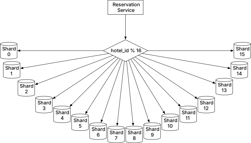
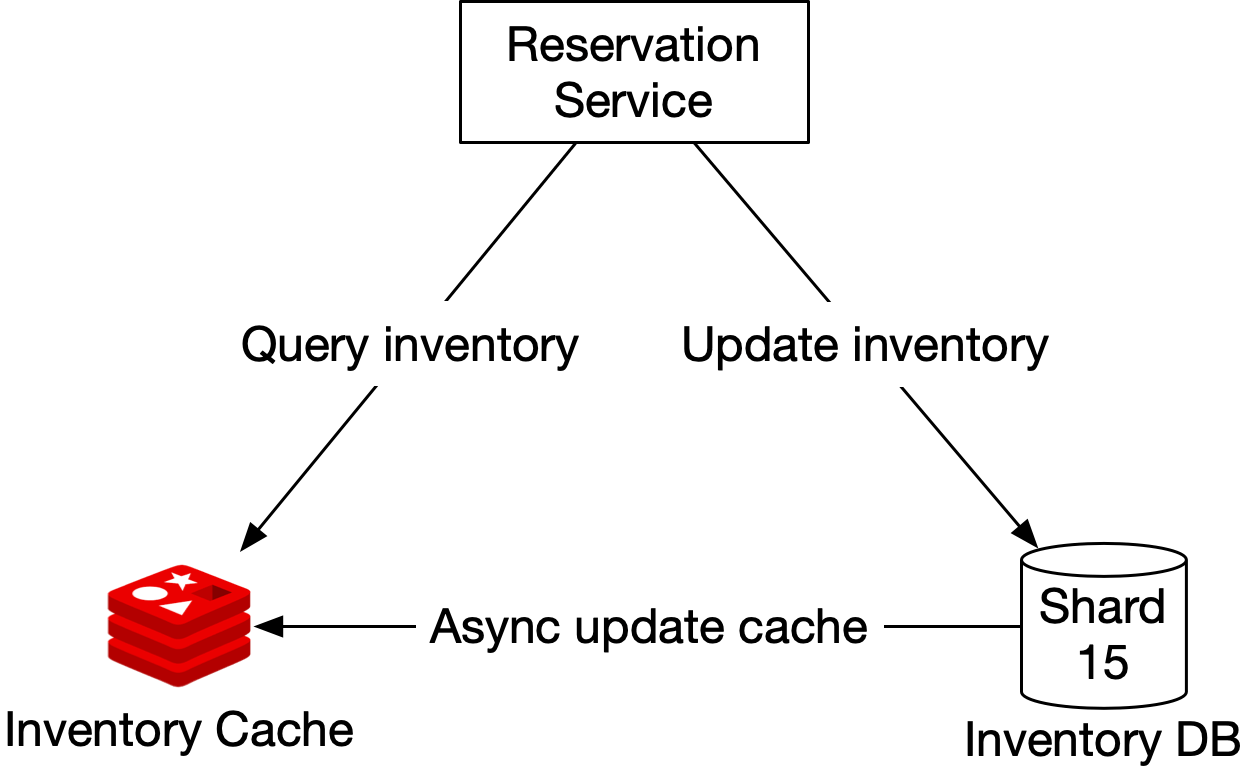
Data consistency among services
**Pragmatic approach (our design):** Reservation Service handles both reservation and inventory APIs, keeping both tables in the **same relational database**. This leverages ACID properties to handle concurrency elegantly.
**Pure microservice alternative (Figures 17-19):** Each service has its own DB. A single logical operation (reserve room + record payment) spans multiple services → cannot use a single transaction.
**Problem (Figure 19):** If inventory update succeeds but reservation DB fails, we need compensating transactions to roll back the inventory change. Many failure cases → data inconsistency.
**Industry techniques for distributed consistency:** - **Two-phase commit (2PC):** Atomic commit across multiple nodes (all succeed or all fail). Blocking protocol — single node failure blocks progress. Not performant. - **Saga:** Sequence of local transactions. Each step publishes a message to trigger the next. On failure, compensating transactions undo prior steps. Relies on eventual consistency (vs. 2PC's strong consistency).
**Decision:** The added complexity of distributed consistency is not worth it for this system. We keep inventory and reservation data in the same relational DB.
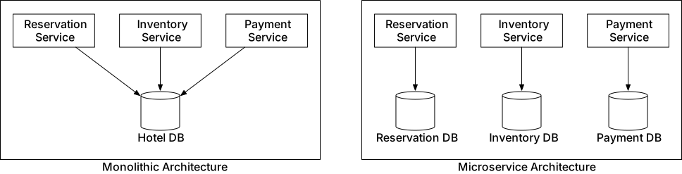
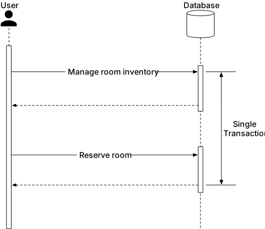
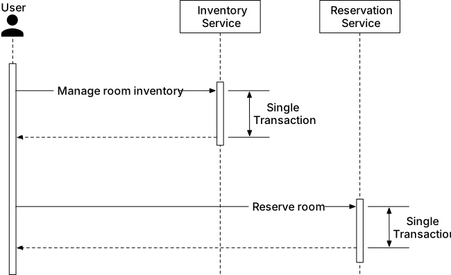
Step 4 - Wrap Up
Key design topics: API design with idempotency keys, room_type_inventory data model, three concurrency solutions (pessimistic locking, optimistic locking, DB constraints), database sharding and Redis caching for scale, 2PC vs Saga for distributed consistency in microservices.
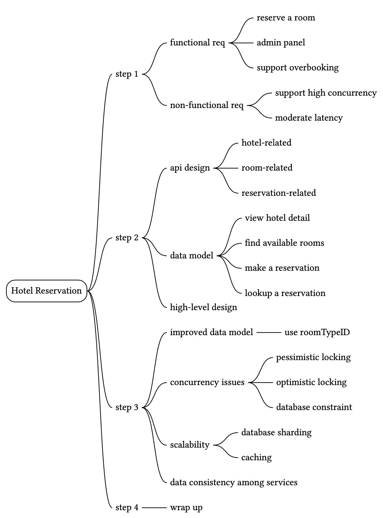
Distributed Email Service
We design a large-scale email service (Figure 1) such as Gmail, Outlook, or Yahoo Mail. In 2020, Gmail had over 1.8 billion active users and Outlook had over 400 million users worldwide.

Step 1 - Understand the Problem and Establish Design Scope
**Scale:** 1 billion users.
**Features in scope:** - Send and receive emails. - Fetch all emails. - Filter emails by read/unread status. - Search emails by subject, sender, and body. - Anti-spam and anti-virus. - Email attachments supported. - HTTP protocol for client-server communication (not legacy SMTP/POP/IMAP for our API).
**Non-functional requirements:** - **Reliability:** No email data loss. - **Availability:** Data automatically replicated across nodes; system functions despite partial failures. - **Scalability:** Handles growing user and email volume without performance degradation. - **Flexibility/Extensibility:** Easy to add features; custom protocols may be needed since legacy POP/IMAP have limited functionality.
**Back-of-the-envelope estimation:** - 1 billion users × 10 emails sent/day ÷ 10⁵ seconds = **100,000 QPS** for sending. - 1 billion users × 40 emails received/day × 365 days × 50 KB metadata = **730 PB metadata/year**. - Attachments: 1 billion × 40 × 365 × 20% × 500 KB = **1,460 PB/year**. - Conclusion: distributed database solution required.
Step 2 - Propose High-Level Design and Get Buy-In
Email knowledge 101
**Email protocols:** - **SMTP** — Standard protocol for sending emails between mail servers. - **POP (Post Office Protocol)** — Downloads emails to local device, deletes from server; single-device access; downloads entire email including large attachments. - **IMAP** — Downloads only headers until opened; emails stay on server; multi-device access; most widely used for individual accounts. - **HTTPS/ActiveSync** — Used for webmail and mobile clients (e.g., Microsoft's proprietary ActiveSync).
**DNS MX records (Figure 2):** Sending servers query DNS for MX records of the recipient's domain. Lower priority number = more preferred. Fallback to higher-priority-number servers if primary is unavailable.
**Email attachments:** Sent via Base64 encoding using MIME (Multipurpose Internet Mail Extension). Size limits: Gmail 25 MB, Outlook 20 MB.
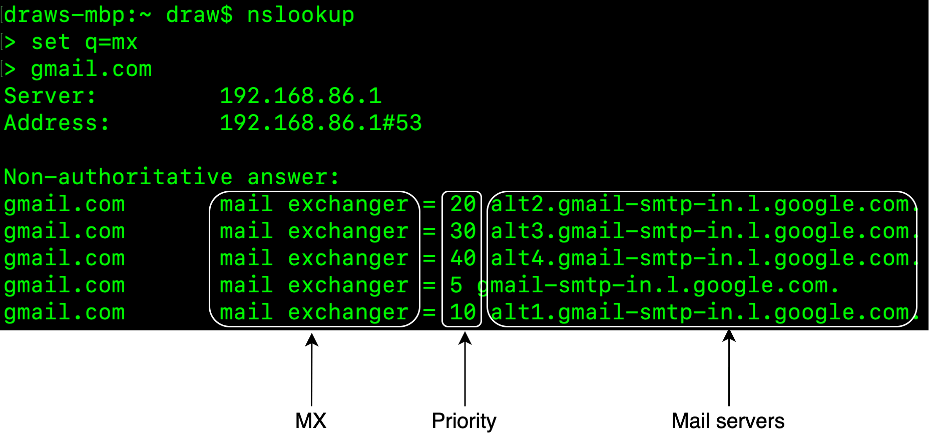
Traditional mail servers
**Traditional flow (Figure 3):** Alice (Outlook) → SMTP → Outlook server → DNS → Gmail SMTP server → stored → IMAP/POP → Bob's Gmail client.
**Storage (Figure 4):** Emails stored in local file directories (one file per email). **Maildir** format was popular. Limitations: - Poor scalability for billions of emails. - Complex file structure → disk I/O bottleneck. - No high availability — disk damage or server failures cause data loss.
Traditional protocols (POP, IMAP, SMTP) were not designed for modern features (threading, labels, search) or billions of users.
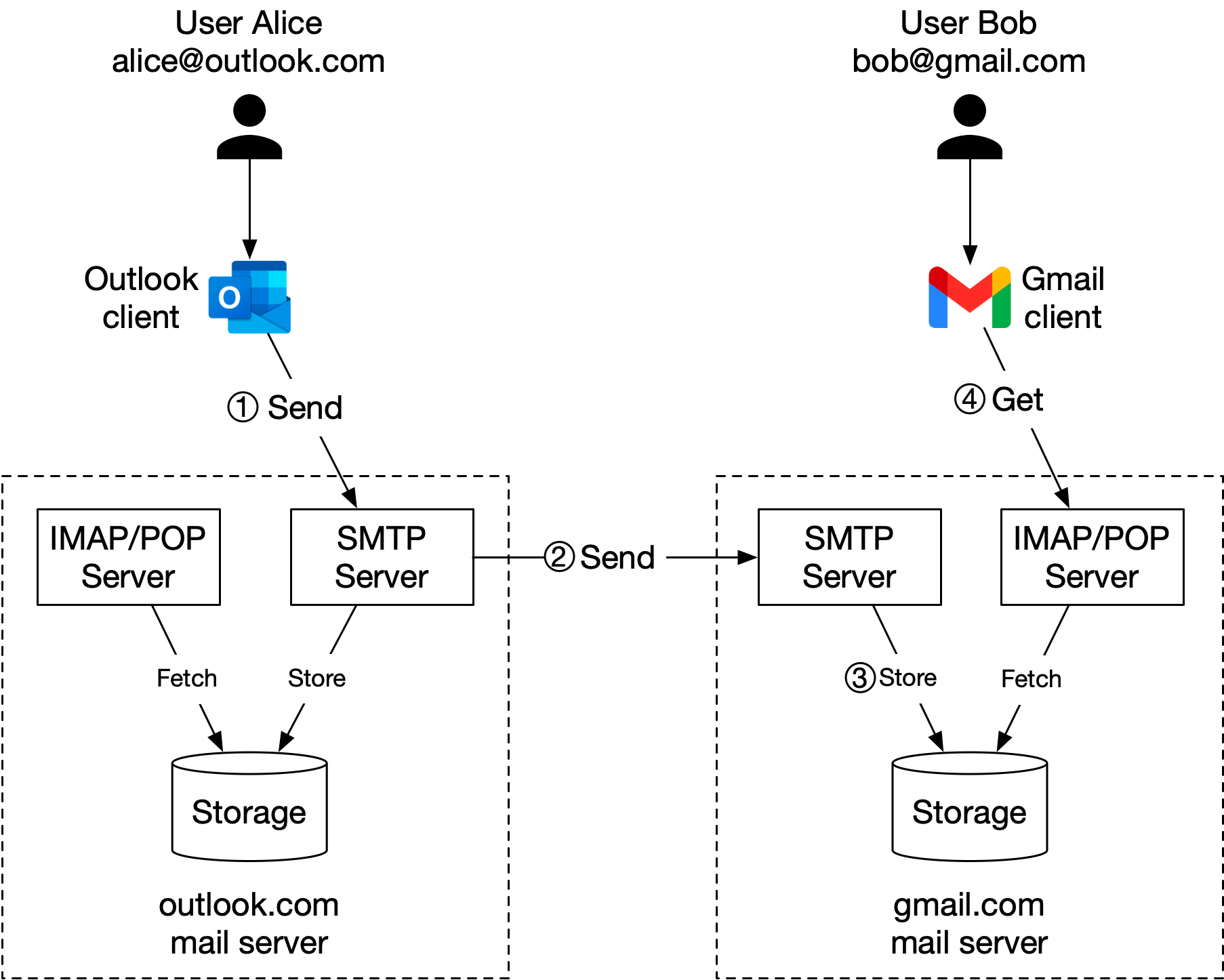

Distributed mail servers
**Email APIs (HTTP/RESTful for webmail):** - `POST /v1/messages` — Send email to To, Cc, Bcc recipients. - `GET /v1/folders` — Get all folders (All, Archive, Drafts, Flagged, Junk, Sent, Trash). - `GET /v1/folders/{folder_id}/messages` — List all messages in a folder (paginated). - `GET /v1/messages/{message_id}` — Get full message details (from, to, subject, body, is_read, attachments).
**High-level design components (Figure 5):** - **Webmail** — Browser-based UI. - **Web servers** — Public-facing: login, signup, profile, all email API requests. - **Real-time servers** — Stateful WebSocket servers that push new emails to online clients. Long-polling as fallback for browser compatibility. - **Metadata database** — Stores email subject, body, from/to, timestamps. Custom or Cassandra-like NoSQL. - **Attachment store** — Amazon S3 (object store). Up to 25 MB attachments. Cassandra not suitable (practical blob limit <1 MB, cache issues). - **Distributed cache** — Redis for caching recent emails (most reads are for recent messages). - **Search store** — Inverted index for full-text search.
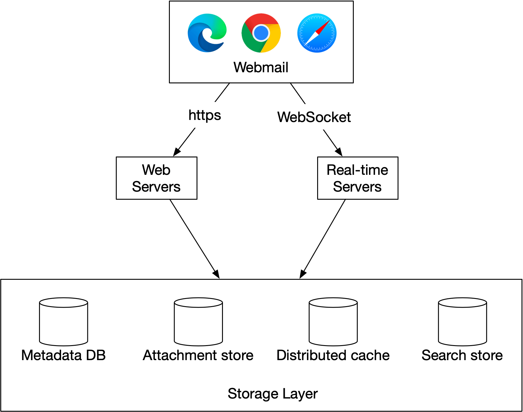
Email sending flow
**Flow (Figure 6):** 1. User clicks "send" → request goes to load balancer. 2. Load balancer enforces rate limiting → routes to web servers. 3. Web server: - 3a. Validates email (size limits, format). - 3b. If same domain: spam/virus check → store in sender's Sent folder + recipient's Inbox directly (no external SMTP needed). 4. Message queues: - 4a. Valid email → outgoing queue (large attachments stored in S3 with reference). - 4b. Invalid email → error queue. 5. SMTP outgoing workers pull from queue → spam/virus check. 6. Email stored in sender's Sent folder. 7. SMTP workers deliver email to recipient's mail server.
**Queue benefits:** Decouples web servers from SMTP workers; enables independent scaling; buffers traffic spikes.
**Queue monitoring:** Stuck emails → diagnose cause: recipient server unavailable (use exponential backoff retry), or insufficient consumers (add more).
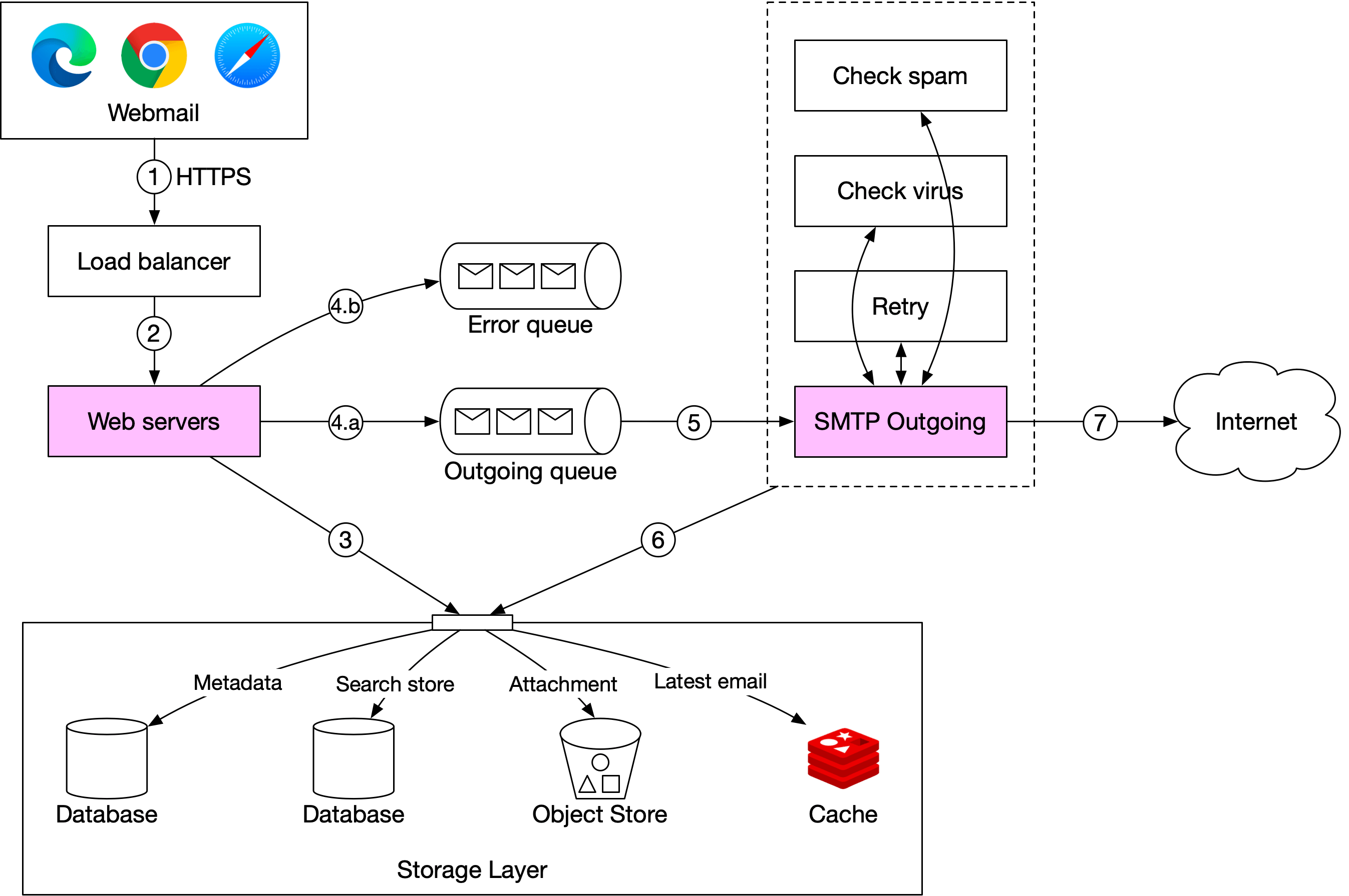
Email receiving flow
**Flow (Figure 7):** 1. Incoming email arrives at SMTP load balancer. 2. Load balancer distributes to SMTP servers; invalid emails bounced at SMTP-connection level. 3. Large attachments stored in S3 before queuing. 4. Email put in incoming queue (buffers surges, decouples from SMTP servers). 5. Mail processing workers filter spam/viruses. 6. Email stored in metadata DB, Redis cache, and S3 (attachments). 7. If receiver is online → pushed to WebSocket real-time servers. 8. WebSocket servers deliver to client in real-time. 9. Offline users: email waits in storage; client fetches via RESTful API on reconnect.
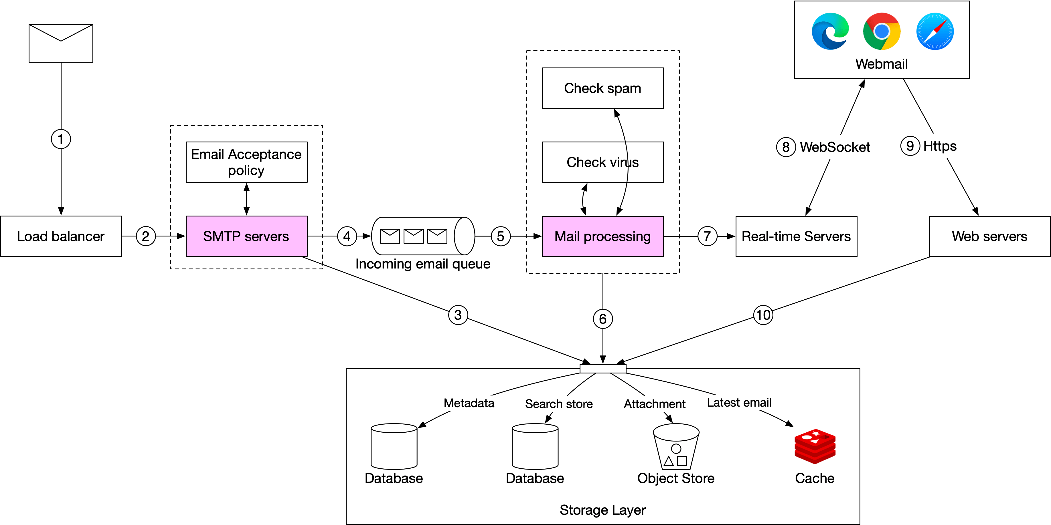
Step 3 - Design Deep Dive
Metadata database
**Characteristics of email metadata:** - Email headers: small, frequently accessed. - Email bodies: larger, read infrequently (usually once). - Mail operations are per-user (no cross-user access). - Data recency: 82% of reads are for emails younger than 16 days. - High reliability: data loss unacceptable.
**Database choices:** - **Relational (MySQL/PostgreSQL):** Good indexing but optimized for small data entries; email bodies (>100 KB HTML) are poor fit; BLOB search is inefficient. - **Distributed object storage (S3):** Good backup, but can't efficiently support read/search/threading operations. - **NoSQL (Bigtable, Cassandra):** Bigtable used by Gmail but not open source; Cassandra possible but no known major email provider uses it.
**Custom database requirements (interview answer):** - Single column can be single-digit MB. - Strong data consistency. - Designed to reduce disk I/O. - Highly available and fault-tolerant. - Easy incremental backups.
**Data model — partition by user_id so all user data is on one shard:**
**Table 1 — Folders by user** (partition key: user_id): - Supports: get all folders for a user.
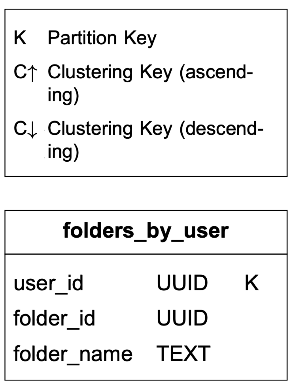
Data model — queries
**Table 2 — Emails by folder** (composite partition key: user_id + folder_id, clustering key: email_id as TIMEUUID for chronological ordering): - Supports: list all emails in a folder sorted by time.
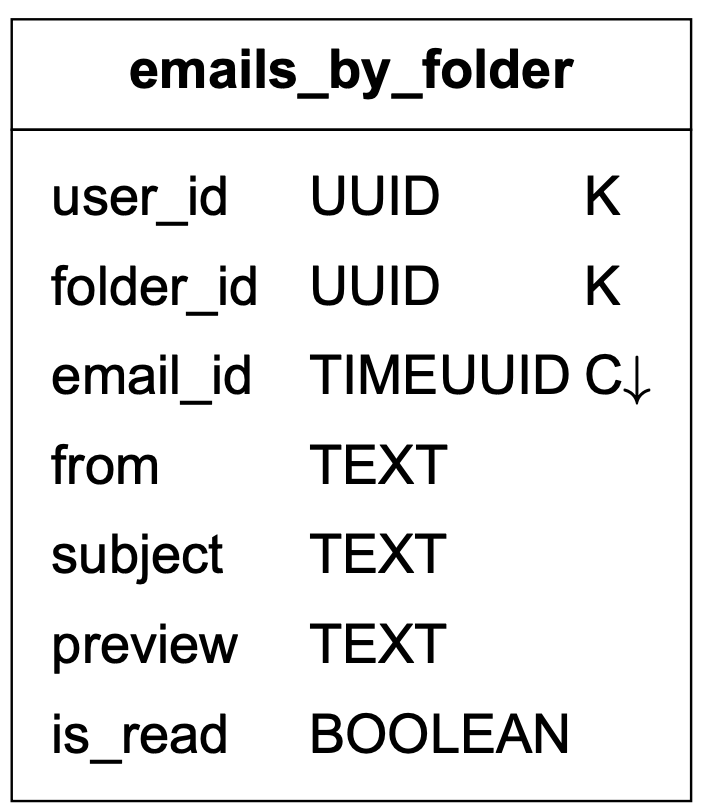
Query 3 — Get email details
**Table 3 — Emails by user** — full email data including attachments (retrieved by email_id + filename).
```sql SELECT * FROM emails_by_user WHERE email_id = 123; ```
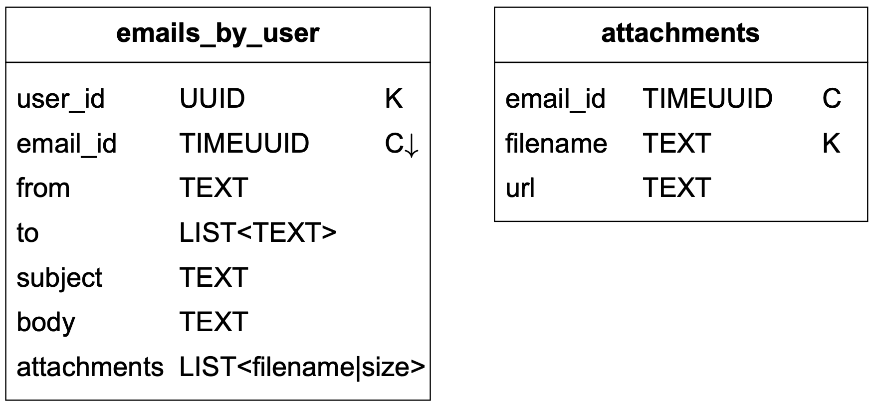
Query 4 — Read/unread emails (NoSQL denormalization)
In NoSQL, `is_read` is not a partition or clustering key → can't filter efficiently. Solution: **denormalization** into two tables (Table 4): - `read_emails` — stores all read emails. - `unread_emails` — stores all unread emails.
To mark as read: delete from `unread_emails`, insert into `read_emails`.
```sql SELECT * FROM unread_emails WHERE user_id = <id> AND folder_id = <id> ORDER BY email_id; ```
Trade-off: more complex application code, better read performance at scale.
**Bonus: Conversation threads** — Use email header fields (Message-Id, In-Reply-To, References) with JWZ algorithm to reconstruct thread chains from preloaded reply chain messages.
**Consistency trade-off:** Single primary per mailbox — trades availability for consistency. During failover, mailbox is inaccessible until failover completes.
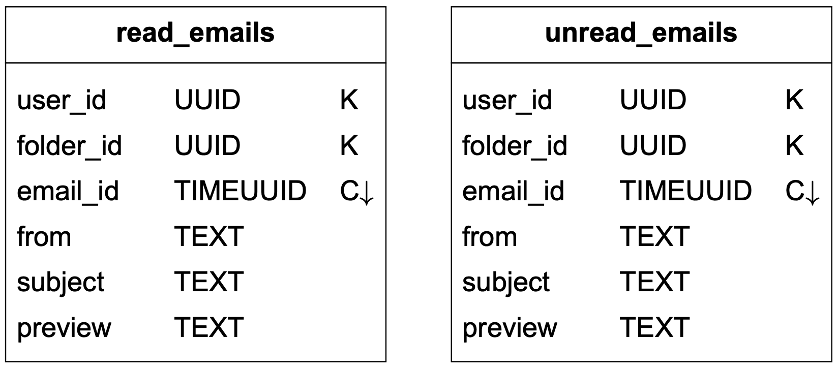
Email deliverability
Getting emails to users' inboxes (not spam) is hard. Over 50% of all emails sent are spam.
**Key factors:** - **Dedicated IPs** — New IP addresses have no reputation; use dedicated IPs with history. - **Classify emails** — Separate IPs for marketing vs transactional emails to avoid spam classification. - **Warm up new IPs** — Build reputation gradually over 2-6 weeks (per Amazon SES guidance). - **Ban spammers quickly** — Prevent reputation damage before significant impact. - **Feedback processing (Figure 8):** Set up feedback loops with ISPs. Process: - **Hard bounce** — Invalid recipient address. - **Soft bounce** — Temporary delivery failure (ISP busy). - **Complaint** — User clicks "report spam". - Separate queues for soft bounces, hard bounces, complaints for independent management.
**Email authentication (Figure 9 — Gmail header example):** - **SPF** (Sender Policy Framework) — Verifies sender IP is authorized to send for the domain. - **DKIM** (DomainKeys Identified Mail) — Cryptographic signature to verify message integrity. - **DMARC** (Domain-based Message Authentication) — Policy framework combining SPF + DKIM.
Phishing and pretexting represent 93% of breaches (Verizon 2018 report).
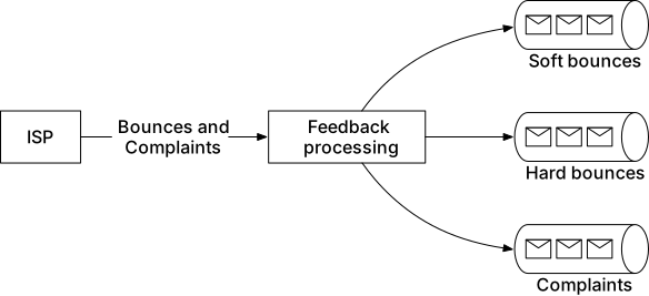
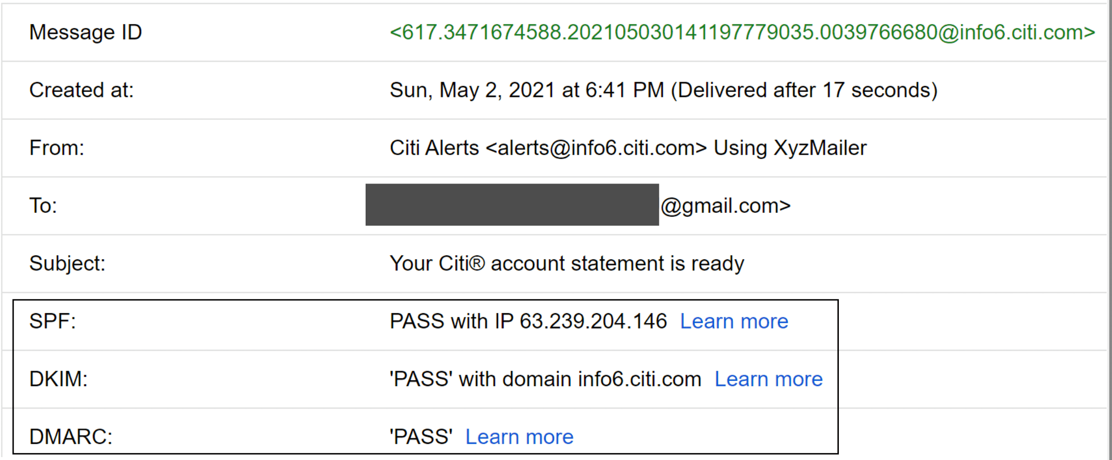
Search
Email search characteristics vs Google search: | Feature | Google Search | Email Search | |---------|--------------|-------------| | Scope | Whole internet | User's own mailbox | | Sorting | By relevance | By time, attachment, unread, etc. | | Accuracy | Some indexing delay acceptable | Near real-time, must be accurate |
Email search is **write-heavy** (reindex on every send/receive/delete); queries are relatively rare.
**Option 1: Elasticsearch (Figure 10)** - Partition underlying documents by user_id → all user data on same node. - Reindexing done asynchronously via offline jobs; Kafka decouples trigger events from reindex workers. - Search requests are synchronous (user waits for results). - Used by Tencent QQ Email at scale.
**Option 2: Custom search with LSM tree (Figure 11)** - For Gmail/Outlook scale, custom search engines are common. - **LSM (Log-Structured Merge-Tree):** Optimized for write-heavy workloads via sequential writes only. - New email → level 0 in-memory cache → merged to next level when threshold reached. - Separates frequently changing data (folder info) from stable data (email content). - Used in BigTable, Cassandra, RocksDB.
| Feature | Elasticsearch | Custom search engine | |---------|--------------|---------------------| | Scalability | Scalable to some extent | Easier (email-specific optimizations) | | Complexity | Two systems (datastore + ES) | One system | | Data consistency | Two copies, hard to sync | Single copy | | Data loss | No (rebuild from primary) | No | | Dev effort | Easy integration | Significant engineering |
**Rule of thumb:** Elasticsearch for smaller scale; native embedded search for Gmail/Outlook scale.
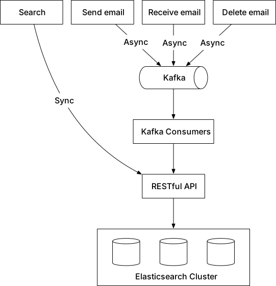
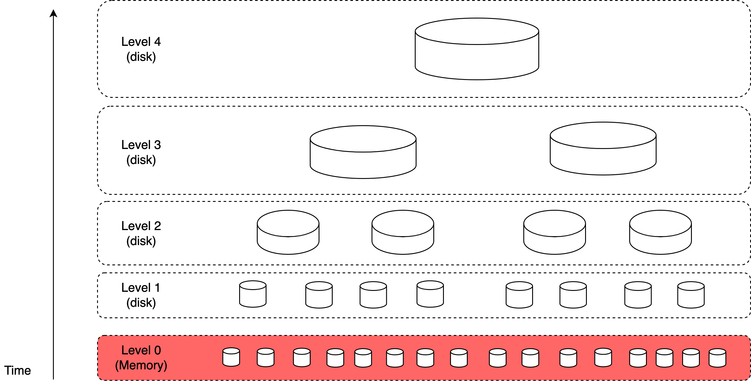
Scalability and availability
Most components are stateless and horizontally scalable (user data access patterns are independent).
For high availability, data replicated across multiple data centers (Figure 12). Users connect to geographically nearest mail server. During network partition, users can still access messages from other data centers.
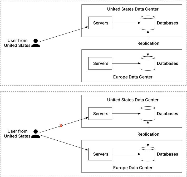
Step 4 - Wrap Up
Key design topics: traditional vs distributed mail server evolution, HTTP API design, email sending/receiving flows with queues, NoSQL data model with denormalization, email deliverability (SPF/DKIM/DMARC), Elasticsearch vs LSM-based custom search, multi-datacenter replication.
Additional talking points: fault tolerance (node failures, network issues), compliance (GDPR, legal intercept), security (Gmail safety features), attachment deduplication (check existence before storing duplicate S3 objects for group emails).
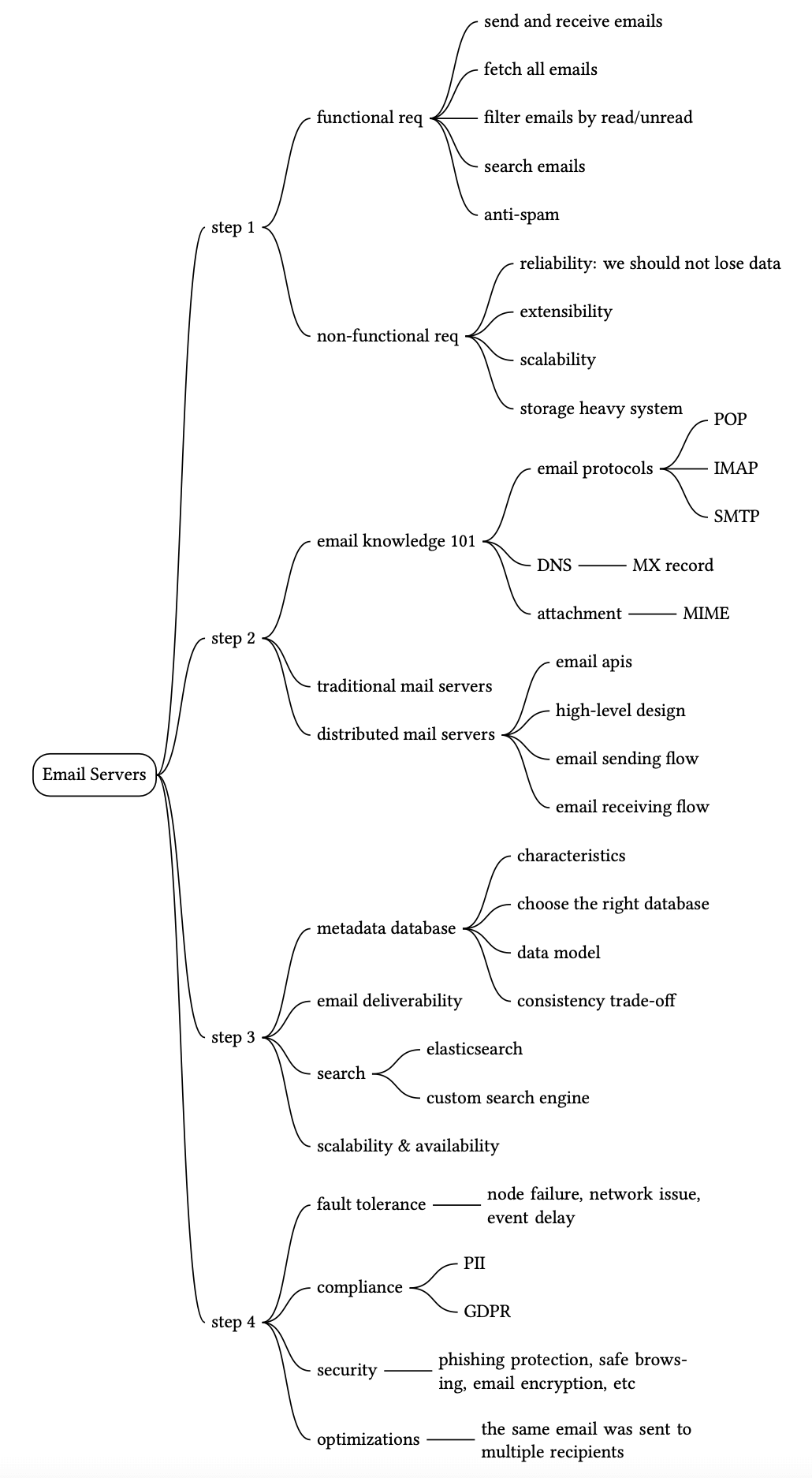
S3-like Object Storage
We design an object storage service similar to Amazon S3. Key milestones: launched 2006, added versioning/multipart upload 2010, 2 trillion objects by 2013, 100 trillion objects by 2021.
Storage System 101
Three broad categories of storage (Figure 1):
**Block storage** (1960s): Physically or network-attached raw blocks (HDD, SSD). Used by VMs, databases, high-performance apps. Accessible via SAS/iSCSI/FC. Mutable, high performance, medium scalability, high cost.
**File storage**: Built on block storage. Hierarchical directory structure. Accessible via SMB/CIFS, NFS. General-purpose. Mutable, medium-high performance and scalability.
**Object storage**: New. Sacrifices performance for high durability, vast scale, low cost. Flat structure (no hierarchy). RESTful API access. Immutable (versioning supported, no in-place update). Used for cold data, archival, backup. AWS S3, Google Cloud Storage, Azure Blob.
**Key S3 terminology:** - **Bucket** — Logical container for objects; globally unique name; must create before uploading. - **Object** — Individual piece of data (payload + metadata key-value pairs). - **Versioning** — Keep multiple variants of an object; enabled per bucket; allows recovery from accidental deletion/overwrite. - **URI** — Each resource (bucket/object) uniquely identified by URI. - **SLA** — S3 Standard-Infrequent Access: 99.999999999% (11 nines) durability, 99.9% availability.
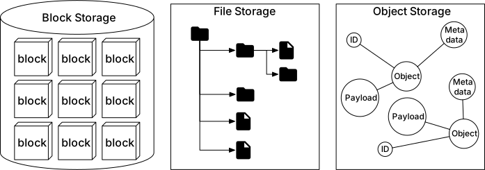
Step 1 - Understand the Problem and Establish Design Scope
**Features:** Bucket creation, object upload/download, object versioning, listing objects in a bucket.
**Data sizes:** Both massive objects (GBs) and many small objects (tens of KB).
**Non-functional requirements:** - **100 PB** data storage. - **6 nines** data durability (99.9999%). - **4 nines** service availability (99.99%). - Storage efficiency: reduce costs while maintaining reliability.
**Back-of-the-envelope estimation:** - Object distribution: 20% small (<1MB), 60% medium (1-64MB), 20% large (>64MB). - Using medians (0.5MB, 32MB, 200MB) at 40% storage usage: - 10¹¹ × 0.4 / (0.2×0.5 + 0.6×32 + 0.2×200) ≈ **0.68 billion objects**. - Metadata at 1KB/object: **0.68 TB** for all metadata. - IOPS bottleneck: spinning disk (7200 rpm SATA) ≈ 100-150 IOPS.
Step 2 - Propose High-Level Design and Get Buy-In
**Key properties of object storage:** - **Immutability** — Objects can be deleted or replaced entirely, but not incrementally modified. - **Key-value store** — URI is the key, object data is the value. - **Write once, read many** — 95% of requests are reads (LinkedIn research). - **Supports small and large objects.**
**Analogy to UNIX file system (Figure 2):** - UNIX: filename in inode → inode has block pointers → data on disk. - Object storage: object name in metadata store → metadata maps to object ID → data in data store via network. - Metadata store ≈ inode (mutable). Data store ≈ disk (immutable once written). - Separation enables independent optimization of each component.
Figure 3 shows the bucket and object relationship.
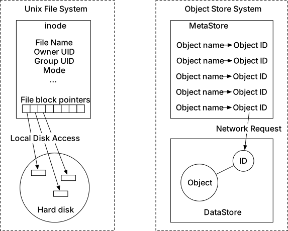
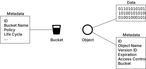
High-level design
**Components (Figure 4):** - **Load balancer** — Distributes RESTful API requests across API servers. - **API service** — Stateless orchestrator; calls IAM, metadata store, and data store. Horizontally scalable. - **IAM (Identity and Access Management)** — Authentication (who you are) + Authorization (what you can do). - **Data store** — Stores/retrieves actual object data by UUID. Immutable objects. - **Metadata store** — Stores object metadata (object name, bucket, UUID, timestamps).
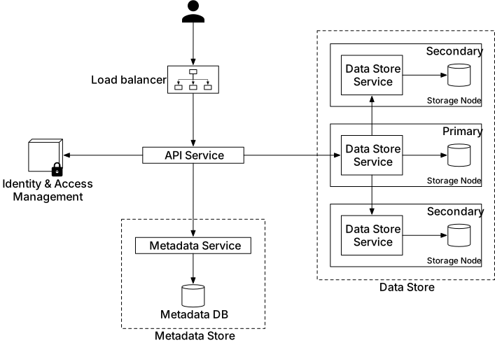
Uploading an object
**7-step upload flow (Figure 5):** 1. Client sends HTTP PUT to create bucket. 2. API service calls IAM to verify WRITE permission. 3. API service creates bucket entry in metadata DB → returns success. 4. Client sends HTTP PUT to upload object (e.g., `script.txt`). 5. API service verifies identity and WRITE permission on bucket. 6. API service sends object data to data store → receives UUID. 7. API service creates metadata entry: `{object_id (UUID), bucket_id, object_name}`.
```http PUT /bucket-to-share/script.txt HTTP/1.1 Content-Type: text/plain Content-Length: 4567 [4567 bytes of object data] ```
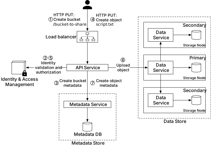
Downloading an object
**Download flow (Figure 6):** 1. Client: `GET /bucket-to-share/script.txt` 2. API service verifies READ permission via IAM. 3. API service fetches object UUID from metadata store (by bucket+object name). 4. API service fetches object data from data store by UUID. 5. Object data returned to client.
Buckets have no directory hierarchy — simulate folders by using `/`-delimited object names (e.g., `abc/d/e/file.txt`).
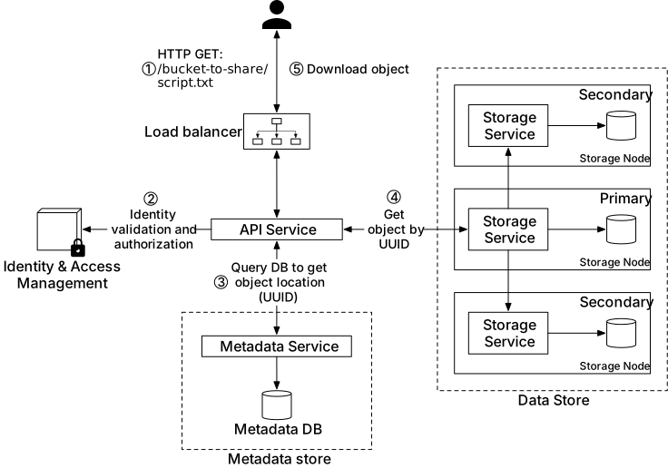
Step 3 - Design Deep Dive
Data store
Figure 7 shows the API service to data store interaction. The data store has three main components (Figure 8):
**Data routing service** — Stateless; queries placement service for best data node; reads/writes data to/from data nodes.
**Placement service** — Determines which data nodes (primary + replicas) store each object. Maintains **virtual cluster map** (Figure 9) with physical topology. Monitors nodes via heartbeats (15s grace period). Critical service — cluster of 5-7 nodes using Paxos or Raft consensus.
**Data node** — Stores actual object data. Runs data service daemon; sends heartbeats to placement service (disk count, data per drive). Replicates data to replication group members for reliability.
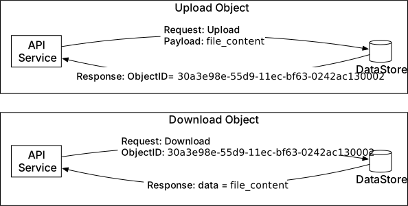
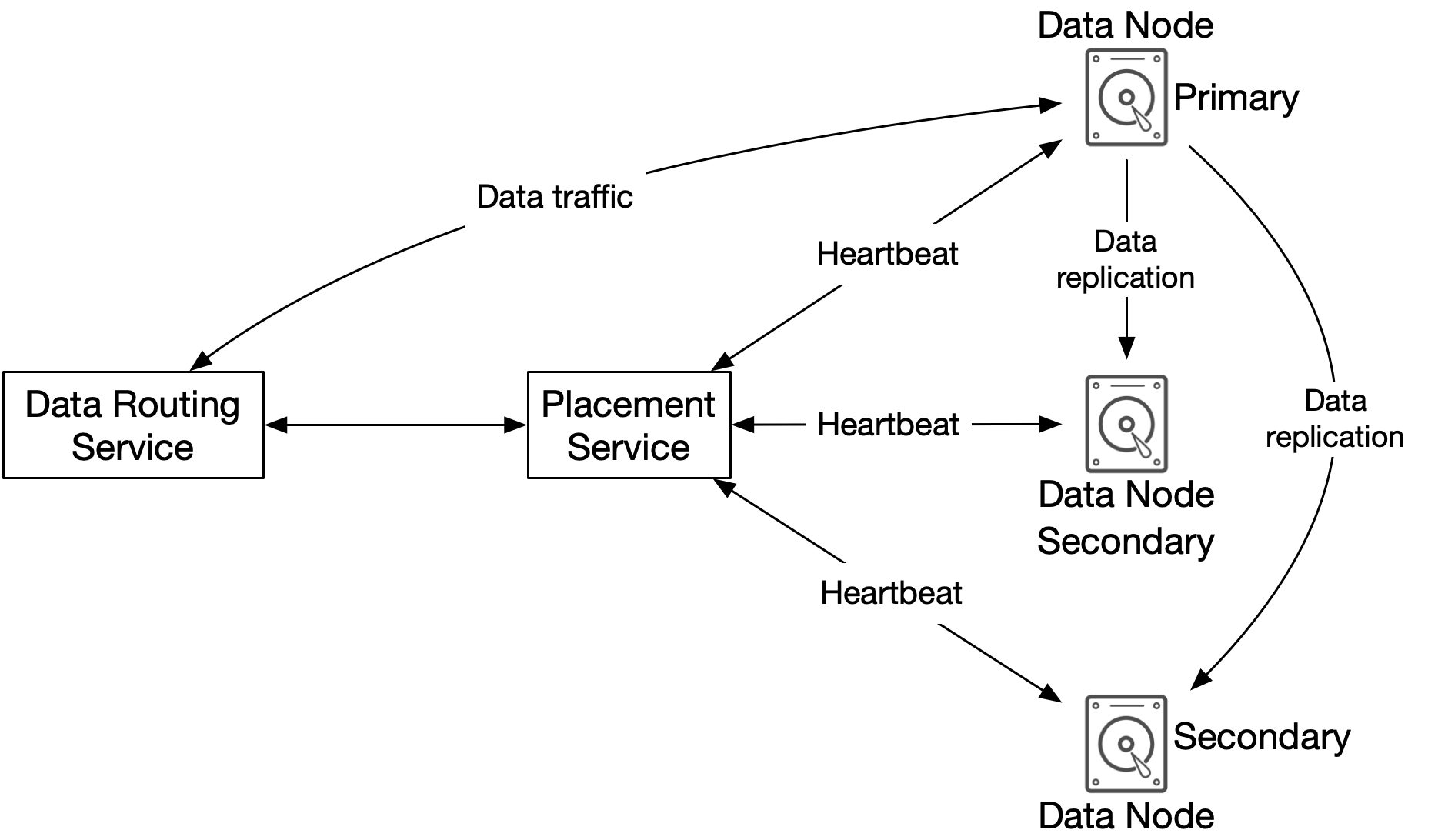
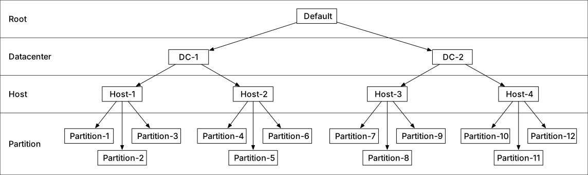
Data persistence flow
**5-step persistence flow (Figure 10):** 1. API service sends object data to data store. 2. Data routing service generates UUID, queries placement service → gets primary data node (via consistent hashing). 3. Data routing service sends data + UUID to primary data node. 4. Primary saves locally and replicates to 2 secondary nodes; responds only after all replicas confirm. 5. UUID returned to API service.
**Consistency vs latency trade-off (Figure 11):** - All 3 nodes save → best consistency, highest latency. - Primary + 1 secondary → medium consistency + latency. - Primary only → worst consistency, lowest latency (options 2 and 3 are eventual consistency).
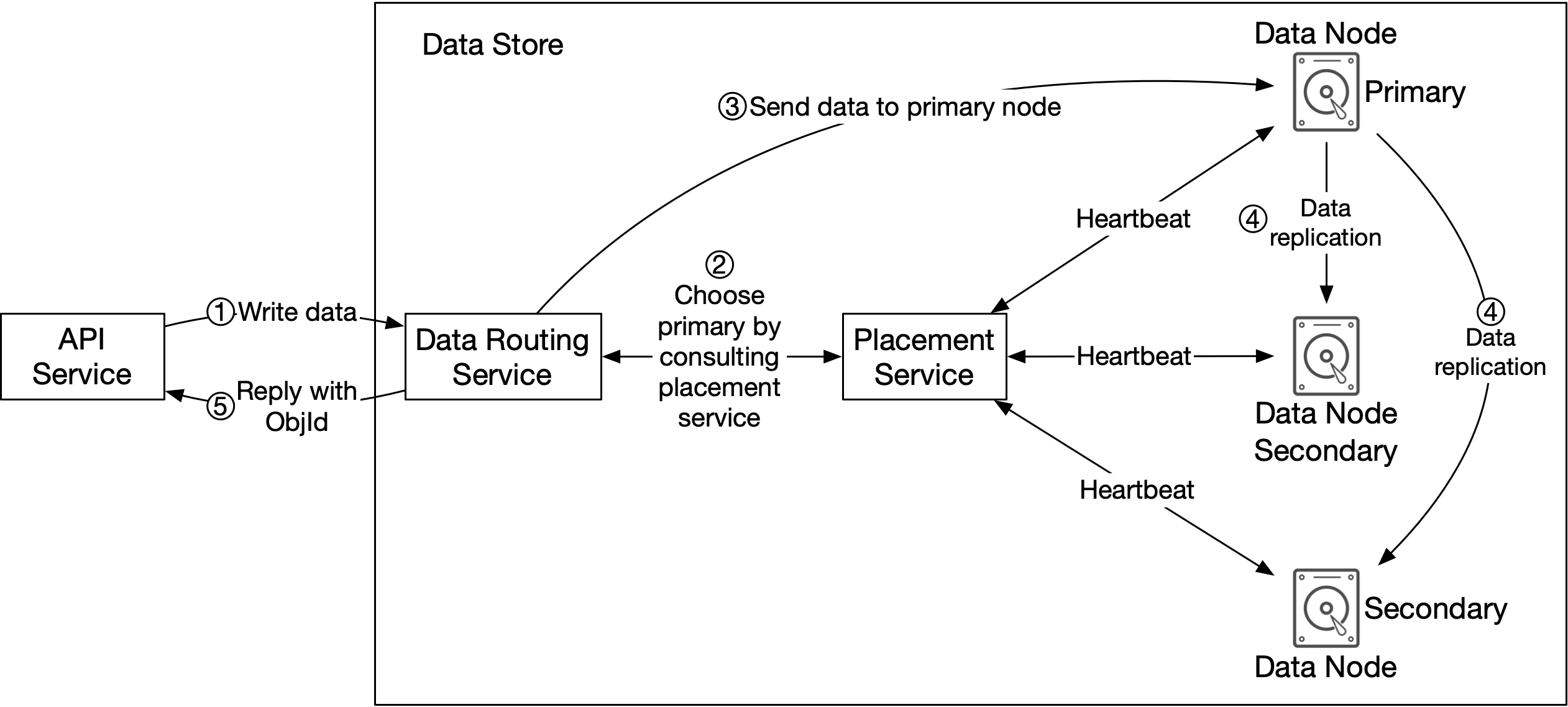
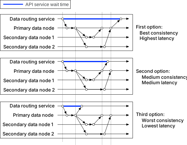
How data is organized
**Problem with one-file-per-object:** Wastes disk blocks (4 KB minimum) for small files; risks exhausting inode capacity; OS handles large inode counts poorly.
**Solution: Merge small objects into large files (Figure 12)** — Works like a write-ahead log (WAL): - Objects appended sequentially to a read-write file. - When file reaches threshold (few GBs) → marked read-only, new read-write file created. - Read-only files serve only reads. - Write access to read-write file is serialized; use one file per CPU core to improve throughput.
**Object lookup** — Data node stores mapping in a local SQLite database (Table 3): | Field | Description | |-------|-------------| | object_id | UUID | | file_name | Data file containing the object | | start_offset | Byte offset in file | | object_size | Object size in bytes |
SQLite chosen over RocksDB: B+ tree provides better read performance (write-once, read-many pattern).
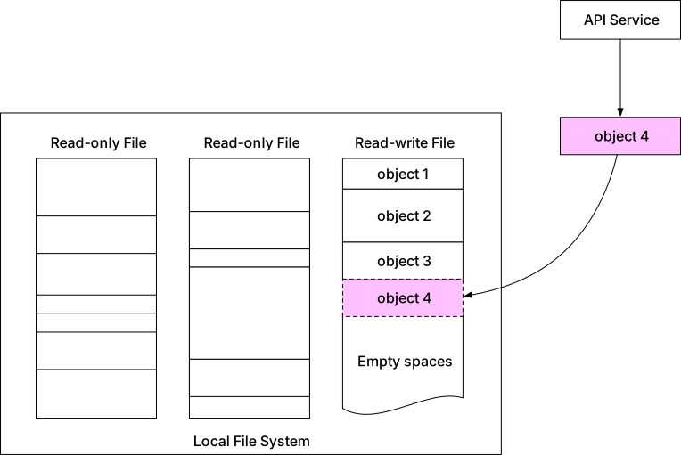
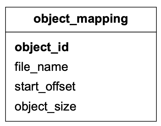
Updated data persistence flow
**Updated 4-step flow (Figure 13):** 1. API service requests save of "object 4". 2. Data node appends object 4 to end of read-write file `/data/c`. 3. New record inserted into `object_mapping` table (SQLite). 4. UUID returned to API service.
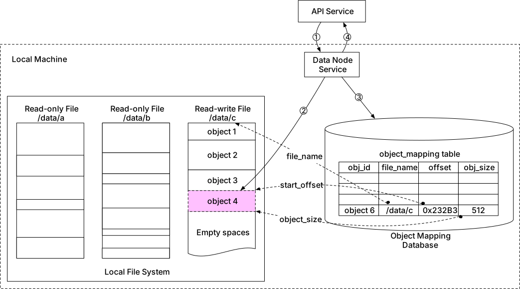
Durability
**3-copy replication:** Annual disk failure rate ~0.81% → 1-(0.0081)³ ≈ **6 nines durability**.
**Failure domains:** Rack-level, node-level failure domains. Replicas placed in different Availability Zones (Figure 14) for isolation against large-scale failures (power outages, natural disasters).
**Erasure coding (Figure 15 — 4+2 example):** - Data split into 4 chunks (d1-d4). - 2 parity chunks calculated (p1, p2) using mathematical formula. - Can reconstruct original data if any 2 chunks are lost.
**8+4 erasure coding (Figure 16):** 12 chunks across 12 failure domains; tolerates any 4 node failures.
**Storage overhead comparison (Figure 17):** - 3-copy replication: **200% overhead**. - 8+4 erasure coding: **50% overhead**. - Erasure coding achieves **11 nines durability** vs 6 nines for replication.
**Replication vs erasure coding trade-offs:** | | Replication | Erasure coding | |--|------------|---------------| | Durability | 6 nines | 11 nines | | Storage overhead | 200% | 50% | | Compute | None | Higher (parity calc) | | Write performance | Faster | Slower (calc parities) | | Read performance | Fast (single node) | Slower (8+ nodes, reconstruct on failure) |
**Rule:** Replication for latency-sensitive apps; erasure coding for cost-optimized storage.
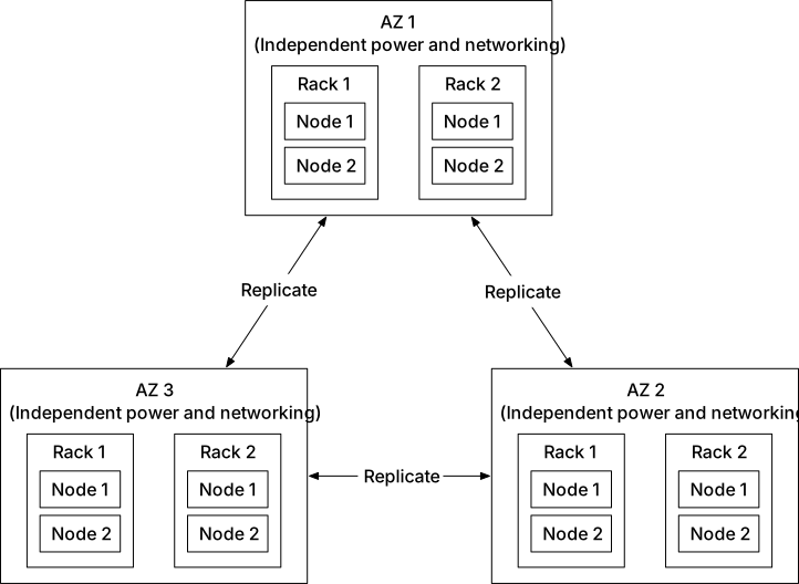
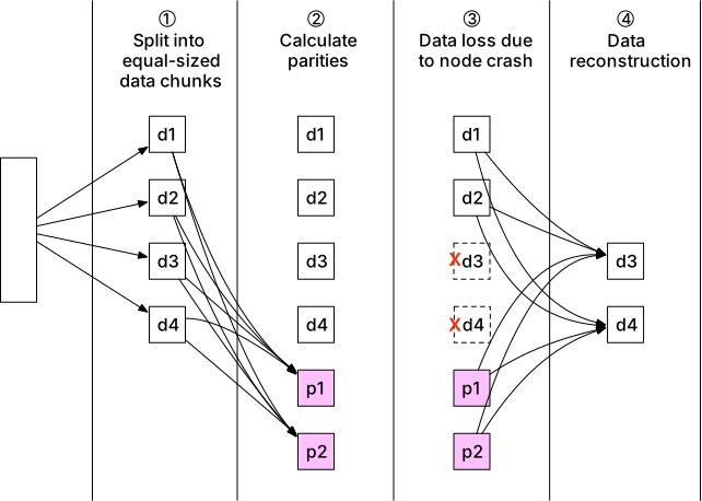
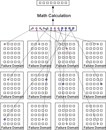
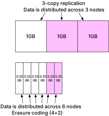
Correctness verification (checksums)
In-memory data corruption is common in large-scale systems. Detect via checksums.
**Checksum generation (Figure 18):** Computed from object data using MD5, SHA1, or HMAC. Good algorithms produce significantly different outputs for even small input changes.
**Checksum comparison (Figure 19):** After transmission, recompute and compare: - Match → data intact. - Mismatch → data corrupted → read from another failure domain.
**Layout (Figure 20):** Checksum appended after each object; file-level checksum at end of read-only file.
**With 8+4 erasure coding:** Fetch 8 data chunks + checksums → verify each → reconstruct if corrupted → return to client.


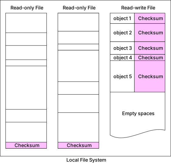
Metadata data model
**Three queries to support:** 1. Find object ID by object name. 2. Insert/delete object by object name. 3. List objects in a bucket sharing a prefix.
**Schema (Figure 21): Two tables — `bucket` and `object`.**
- `bucket` table: small (1M customers × 10 buckets × 1KB ≈ 10 GB). Fits in single DB; scale reads with replicas. - `object` table: massive. Needs sharding.
**Sharding key: hash(bucket_name + object_name)** - Not by bucket_id alone → hotspot risk (buckets with billions of objects). - Not by object_id alone → can't support URI-based queries (most operations use object name). - Combined key → even distribution + URI-based query support.
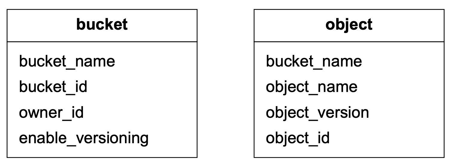
Listing objects in a bucket
S3 uses **prefixes** to simulate directory structure. Object name: `abc/d/e/f/file.txt` → prefix: `abc/d/e/f/`.
**Three listing modes:** 1. `aws s3 list-buckets` — List all buckets owned by user. 2. `aws s3 ls s3://mybucket/abc/` — List at prefix level; deeper paths rolled up to common prefix. 3. `aws s3 ls s3://mybucket/abc/ --recursive` — Recursively list all objects sharing prefix.
**Single database:** Simple LIKE query: `SELECT * FROM object WHERE bucket_id = '123' AND object_name LIKE 'abc/%'`
**Distributed sharded database challenge:** Objects distributed across shards → query all shards, aggregate results. Pagination is complex (each shard has different offset to track).
**Solution for sharded listing:** Denormalize listing data into a separate table sharded by bucket_id. Listing queries hit only this table (single-shard lookup). Object listing performance is not a priority in S3-like systems — all commercial object storage has suboptimal listing performance.
Object versioning
Keeps multiple versions of an object; restores accidentally deleted/overwritten files. Must be enabled per bucket.
**Versioned upload flow (Figure 22):** 1. Client: `PUT script.txt` 2. API service verifies WRITE permission. 3. Data store persists new object → returns new UUID. 4. API service stores metadata. 5. Instead of overwriting: insert new row with same `bucket_id` + `object_name` but new `object_id` and `object_version` (TIMEUUID). Current version = largest TIMEUUID (Figure 23).
**Deleting a versioned object (Figure 24):** All versions remain in bucket; a **delete marker** is inserted as the newest version. GET request on a delete marker returns 404 Object Not Found.
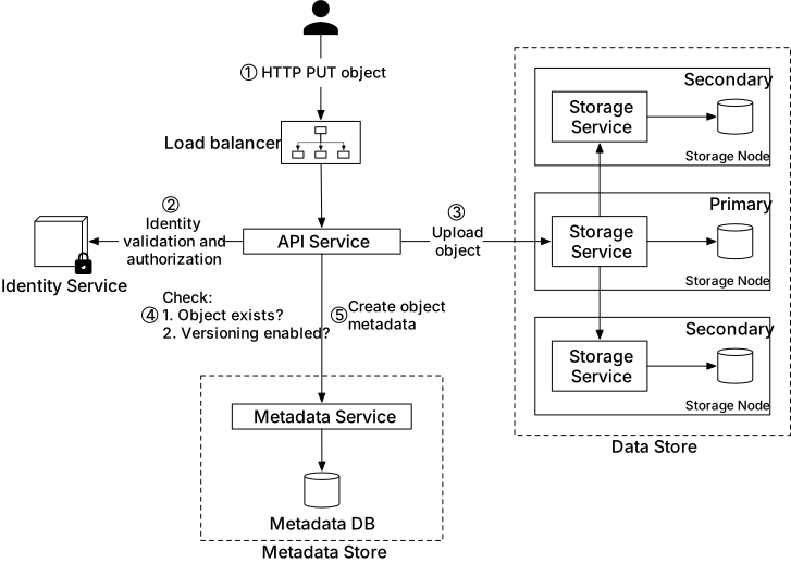
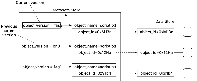
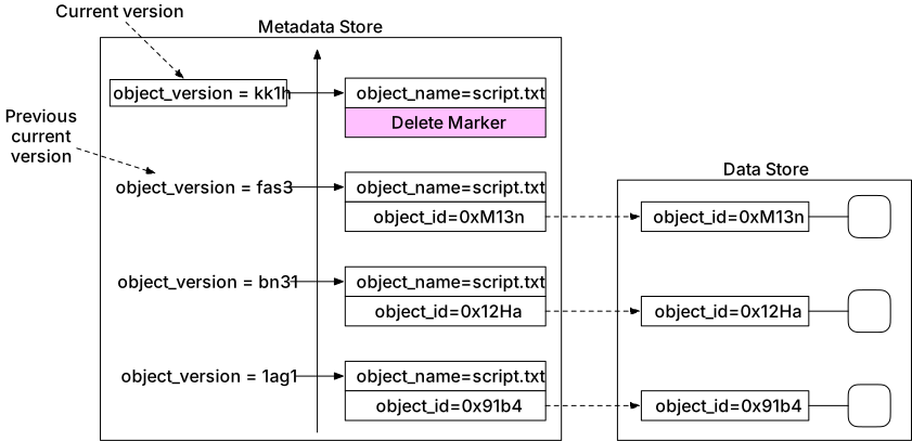
Optimizing uploads of large files (multipart upload)
Large objects (GBs) benefit from parallel chunked upload. Network failure doesn't require restarting entire upload.
**Multipart upload flow (Figure 25):** 1. Client initiates multipart upload → receives `uploadID`. 2. Client splits file (e.g., 1.6 GB into 8 × 200 MB parts). 3. Client uploads each part with `uploadID` → receives **ETag** (MD5 checksum of part). 4. After all parts uploaded, client sends **complete multipart upload** request with `{uploadID, part numbers, ETags}`. 5. Data store reassembles object from parts (may take minutes) → returns success.
Abandoned parts cleaned up by garbage collection service.
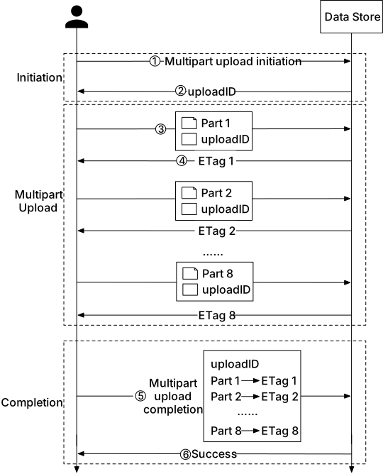
Garbage collection
Reclaims storage no longer in use. Sources of garbage: - **Lazy deletion** — Object marked deleted but not immediately removed. - **Orphan data** — Half-uploaded or abandoned multipart uploads. - **Corrupted data** — Failed checksum verification.
**Compaction mechanism (Figure 26):** 1. Garbage collector copies live objects from old file `/data/b` to new file `/data/d`, skipping objects with `delete_flag = true`. 2. Updates `object_mapping` table (wrapped in DB transaction): updates `file_name` and `start_offset` while preserving `obj_id` and `object_size`. 3. New file is smaller; waits for many read-only files before compacting to avoid creating many small files.
Also reclaims replica space: delete from all 3 copies (replication) or all 12 nodes (8+4 erasure coding).
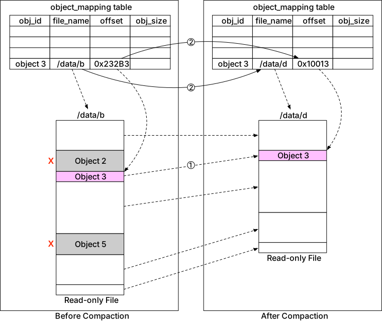
Step 4 - Wrap Up
Key design topics: block/file/object storage comparison, inode analogy for metadata/data separation, upload/download flows, data node organization (WAL-like file merging + SQLite mapping), replication vs erasure coding durability, checksum verification, metadata sharding by (bucket_name + object_name), listing with prefix queries, versioning with TIMEUUID, multipart upload, garbage collection with compaction.
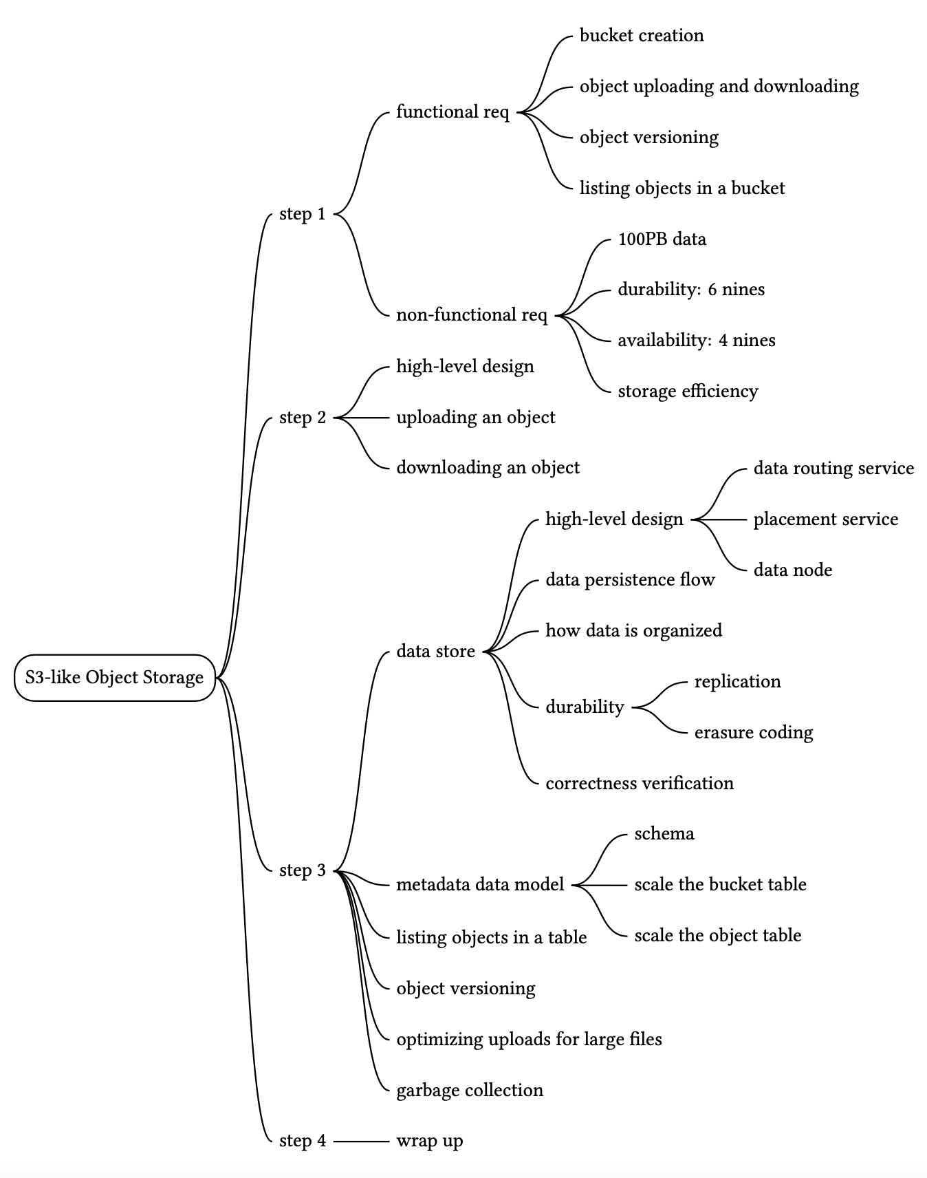
Real-time Gaming Leaderboard
We design a real-time leaderboard for an online mobile game (Figure 1). Leaderboards rank players by points earned from winning matches and display top players and individual user rankings.
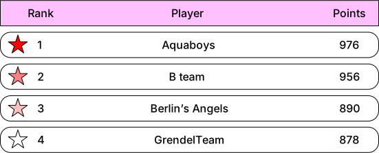
Step 1 - Understand the Problem and Establish Design Scope
**Functional requirements:** - Display **top 10 players** on the leaderboard. - Show a **user's specific rank**. - Bonus: Display players **4 places above and below** a specific user. - Score system: 1 point per match win; monthly tournament resets leaderboard. - Same score → same rank.
**Scale:** - **5 million DAU**, 25 million MAU. - Each player plays ~10 matches/day.
**Non-functional requirements:** - **Real-time** score updates (no batched results acceptable). - General scalability, availability, reliability.
**Back-of-the-envelope estimation:** - Average users/sec: 5M / 10⁵ = **~50 users/sec**; peak (5×) = **250/sec**. - QPS for scoring a point: 50 × 10 = **500 QPS**; peak = **2,500 QPS**. - QPS for fetching top 10: ~**50 QPS** (loaded once per daily session).
Step 2 - Propose High-Level Design and Get Buy-In
API design
**POST /v1/scores** — Update user's score when they win a game. Internal API only (called by game servers, not clients — prevents cheating via man-in-the-middle attacks). ```json { "user_id": "user1", "points": 1 } ```
**GET /v1/scores** — Fetch top 10 players from leaderboard. ```json { "data": [{"user_id": "user1", "user_name": "alice", "rank": 1, "score": 12543}, ...], "total": 10 } ```
**GET /v1/scores/{:user_id}** — Fetch rank of a specific user. ```json { "user_info": { "user_id": "user5", "score": 1000, "rank": 6 } } ```
High-level architecture
**Two services (Figure 2):** 1. **Game service** — Validates match wins, calls leaderboard service to update score. 2. **Leaderboard service** — Updates scores in leaderboard store; serves top 10 and user rank queries.
**Why game server sets scores (not client):** Client-side score setting is vulnerable to man-in-the-middle attacks where players intercept and modify scores.
**Message queue (Figure 4):** Optional Kafka between game and leaderboard services — useful when scores feed multiple consumers (analytics, push notifications, leaderboard). Not required based on stated requirements.
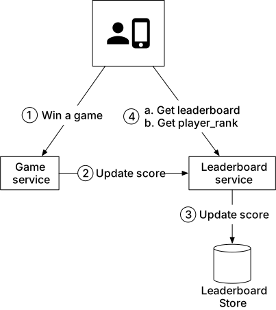
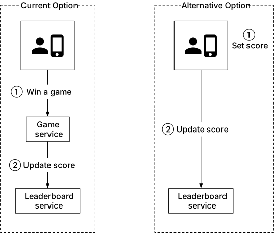
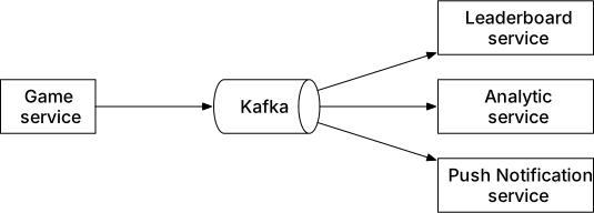
Data models
Relational database solution
**Simple approach (Figure 5):** Monthly leaderboard table with user_id and score columns.
```sql -- User wins a point: INSERT INTO leaderboard (user_id, score) VALUES ('mary1934', 1); UPDATE leaderboard SET score=score+1 WHERE user_id='mary1934';
-- Find user rank (Figure 7): SELECT (@rownum := @rownum+1) AS rank, user_id, score FROM leaderboard ORDER BY score DESC; ```
**Why it fails at scale:** - Finding a user's rank requires sorting the entire table → O(n) scan over millions of rows. - 10s of seconds for rank queries — unacceptable for real-time requirement. - Constantly changing data makes caching infeasible. - Even with index + LIMIT 10, determining rank of non-top users still requires full scan.
**Conclusion:** Relational database works for small datasets or batch operations only.
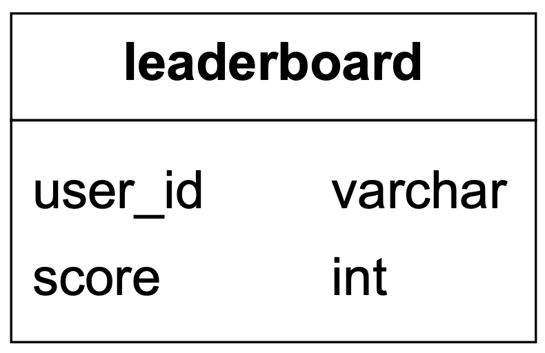


Redis sorted sets solution
**Redis sorted sets** (Figure 8): Each member is unique with an associated score. Internally uses two data structures: - **Hash table** — maps users to scores. - **Skip list** — maps scores to users for fast rank queries.
**Skip list (Figure 9):** Sorted linked list + multi-level indexes. Each level skips every other node of the previous level. Search for a value traverses top index first, dramatically reducing comparisons vs O(n) linked list.
**Figure 10:** Skip list with 5 index levels — finds a node in 11 traversals vs 62 for base linked list.
**All operations are O(log n)** — predictable performance at millions of users.
**Redis commands used:** - `ZADD` — Insert/update user in sorted set. O(log n). - `ZINCRBY <key> <increment> <user>` — Increment user score; adds user at score 0 if not present. O(log n). - `ZRANGE/ZREVRANGE` — Fetch range of users by score (ascending/descending). O(log n + m). - `ZRANK/ZREVRANK` — Get rank of a user. O(log n).
**Workflow:**
1. **User scores a point (Figure 11):** ``` ZINCRBY leaderboard_feb_2021 1 'mary1934' ```
2. **Fetch top 10 (Figure 12):** ``` ZREVRANGE leaderboard_feb_2021 0 9 WITHSCORES ``` Returns: `[(user2,score2),(user1,score1)...]`
3. **Fetch user rank (Figure 13):** ``` ZREVRANK leaderboard_feb_2021 'mary1934' ```
4. **Fetch 4 players above and below rank 361 (Figure 14):** ``` ZREVRANGE leaderboard_feb_2021 357 365 ```
**Storage estimate:** - 25M MAU × 26 bytes/entry (24-char user_id + 2-byte score) = **~650 MB** — fits on a single Redis server. - Peak QPS 2,500 — well within single Redis server capacity.
**Persistence:** Redis configured with read replica; main instance failure → replica promoted.
**Supporting MySQL tables:** `user` (profile data) and `point` (history of wins with timestamps) — used for play history and leaderboard recovery after failure.
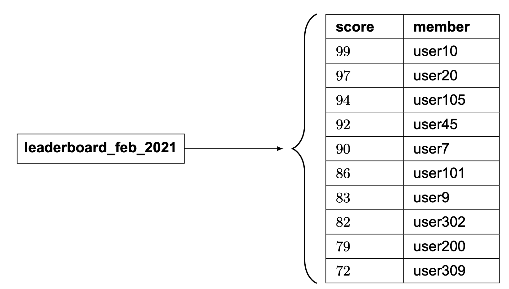
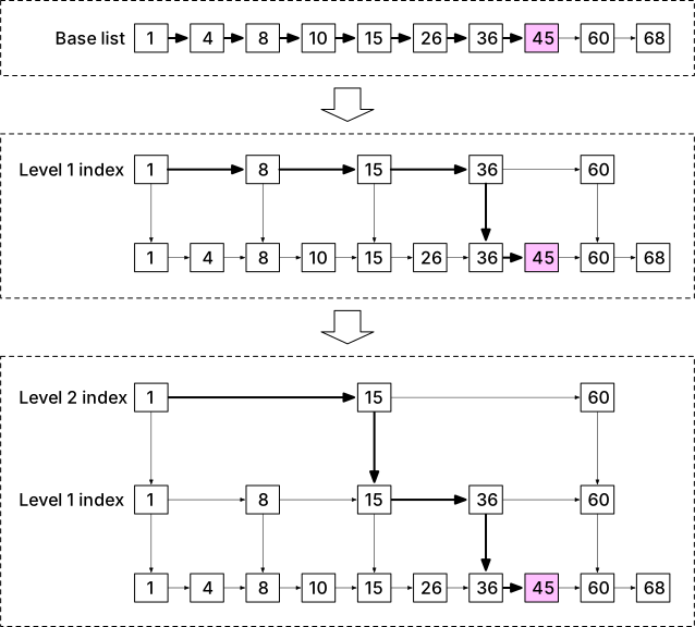




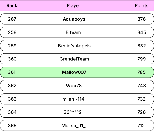
Step 3 - Design Deep Dive
Cloud vs self-managed deployment
**Self-managed (Figure 15):** Monthly sorted set in Redis + MySQL for user profiles. API servers query Redis for leaderboard data + MySQL for user names/images. Optional cache for top 10 user profiles.
**Serverless on AWS (Figures 16-17):** Amazon API Gateway → AWS Lambda functions → Redis + MySQL.
| API | Lambda function | |-----|----------------| | GET /v1/scores | LeaderboardFetchTop10 | | GET /v1/scores/{user_id} | LeaderboardFetchPlayerRank | | POST /v1/scores | LeaderboardUpdateScore |
**Serverless benefits:** No server provisioning, auto-scaling with traffic, no infrastructure maintenance. Recommended for greenfield projects.
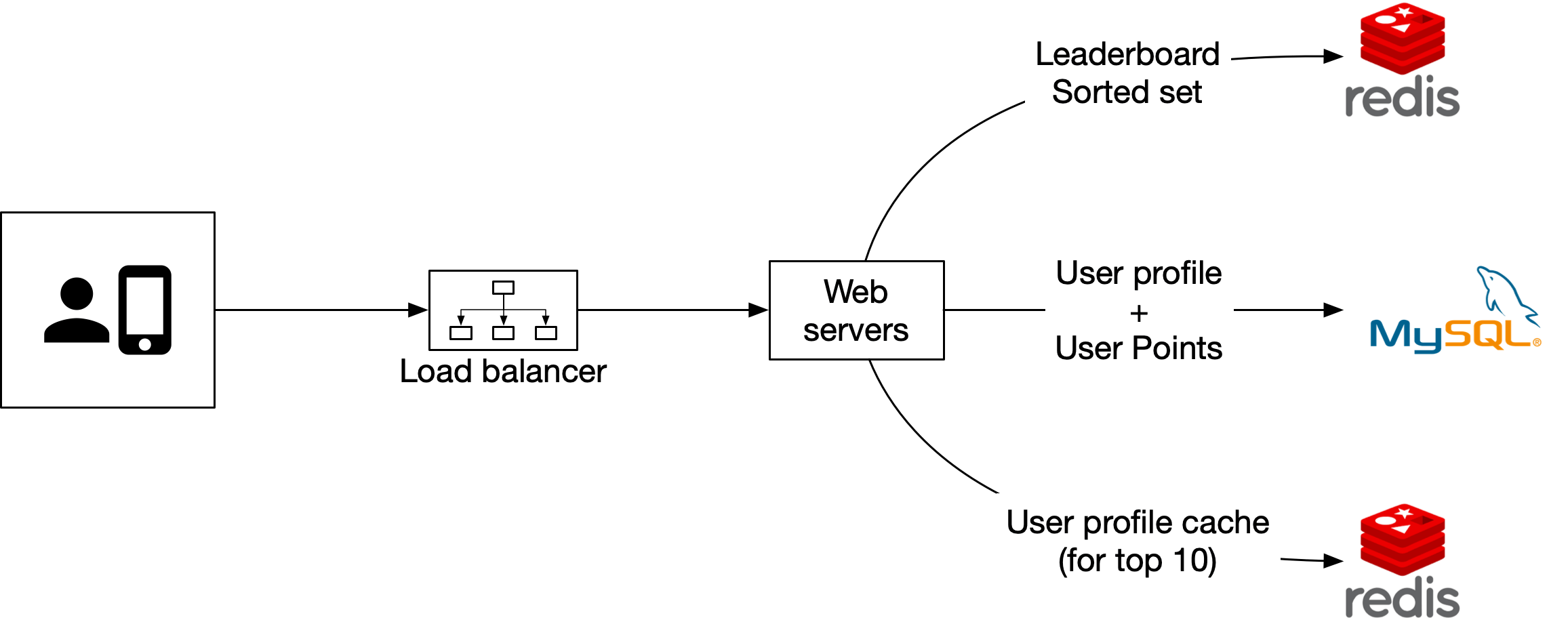
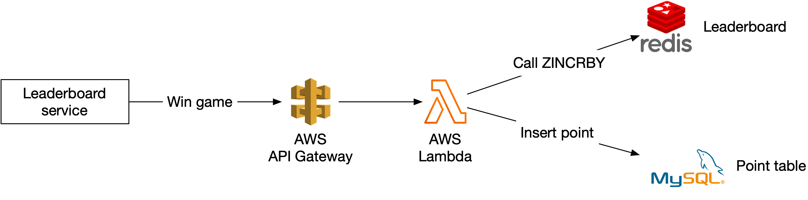
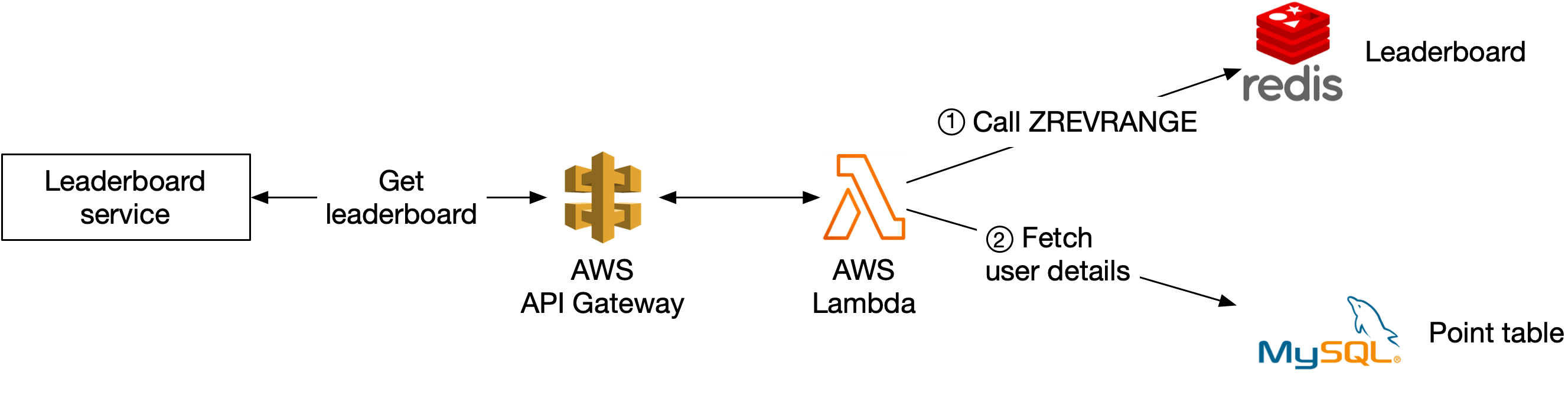
Scaling Redis
At 500M DAU (100× scale): leaderboard grows to **65 GB**, peak QPS **250,000**. Requires sharding.
**Option 1: Fixed partitions (Figure 18)** - Score range 1-1000 → 10 shards, each covering 100-point range. - Application routes to correct shard based on user score. - Need secondary cache: user_id → current score (to know which shard they're in). - Score increase crossing shard boundary → remove from old shard, add to new. - Fetch top 10: query only the highest-score shard. - Fetch user rank: local rank within shard + count of users in higher shards (O(1) via `INFO keyspace`). - **Recommended approach.**
**Option 2: Redis cluster hash partitioning (Figure 19)** - 16,384 hash slots; key assigned via `CRC16(key) % 16384`. - Automatic sharding; easy to add/remove nodes. - Fetch top 10 requires scatter-gather (Figure 20): query all shards, application sorts results. - Limitations: high latency for large K top-K queries; high latency with many partitions; no straightforward user rank determination. - **Not recommended** for this use case.

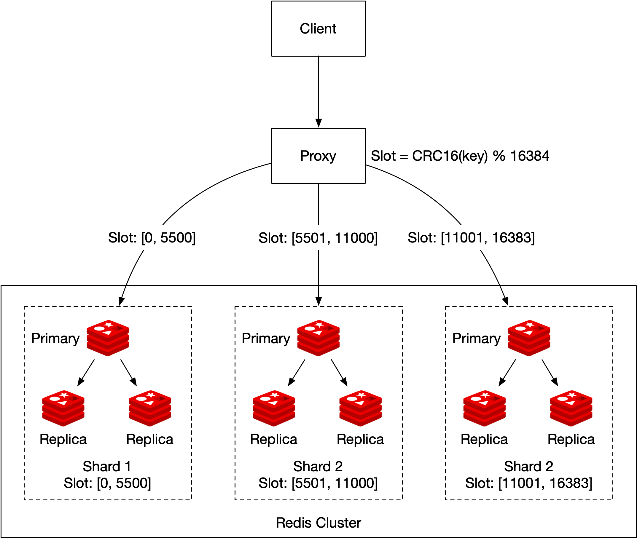
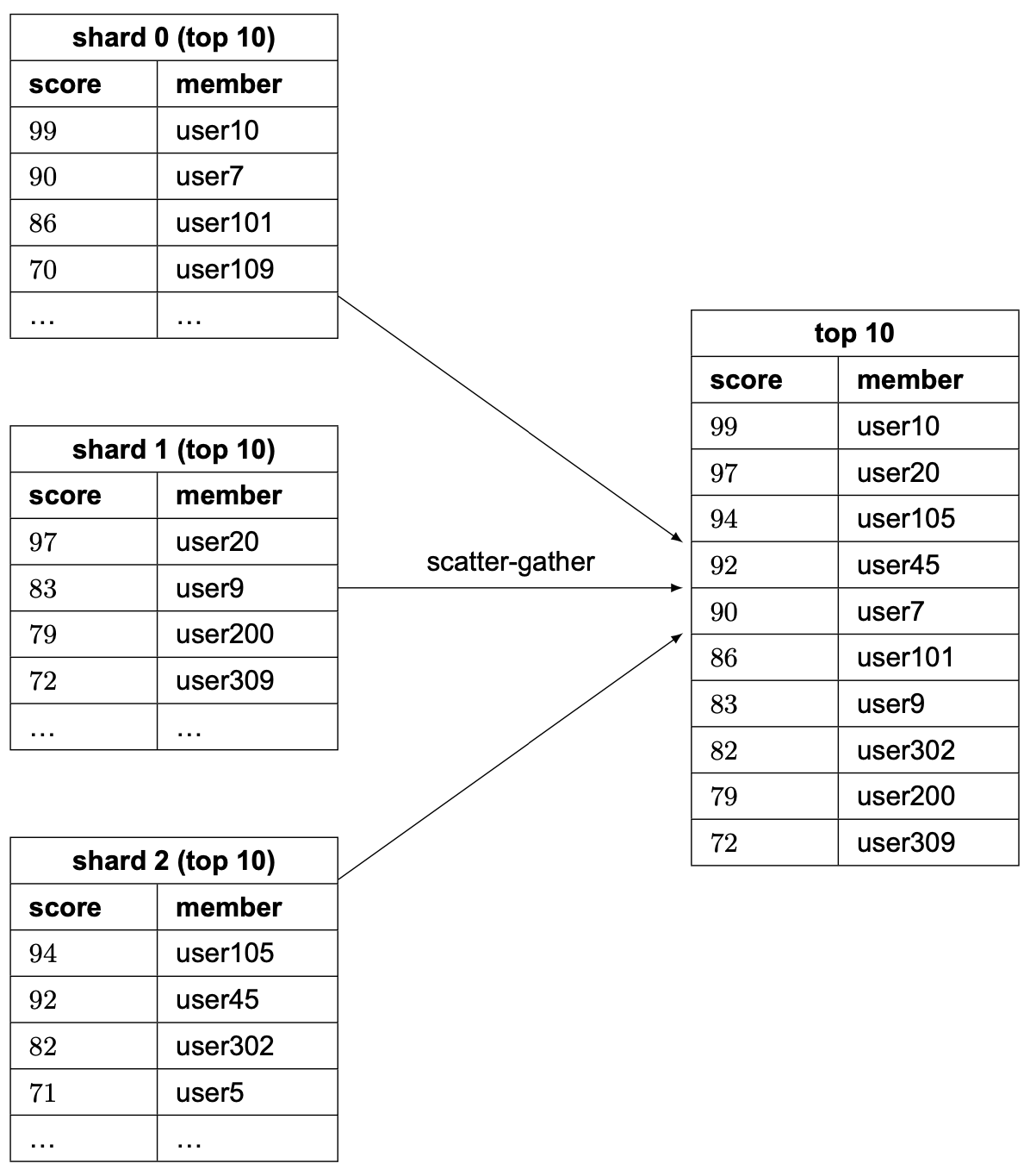
Alternative solution: NoSQL (DynamoDB)
DynamoDB with **Global Secondary Indexes (GSI)** as an alternative to Redis.
**Figure 21:** System diagram with DynamoDB replacing Redis + MySQL.
**Initial table design (Figure 22):** Denormalized leaderboard + user table. Problem: full table scan for top scores.
**First index attempt (Figure 23):** Partition key = `game_name#{year-month}`, sort key = `score`. Problem: all current-month data on one partition → **hot partition**.
**Write sharding solution (Figure 24):** Partition key = `game_name#{year-month}#p{partition_number}` where partition_number = `user_id % N`. Data spread evenly across N partitions.
**Trade-off:** N partitions → lighter per-partition load, but reading top 10 requires **scatter-gather** across all N partitions (Figure 25): 1. Query top 10 from each partition in parallel. 2. Application merges and sorts results.
**User rank limitation:** No straightforward absolute rank. Use **percentile approximation** instead: - Cron job analyzes score distribution per shard → caches percentile thresholds. - Returns "you're in the top 10-20%" instead of exact rank #1,200,001.
**Choosing partition count:** Requires benchmarking — more partitions = lighter load but more scatter complexity.

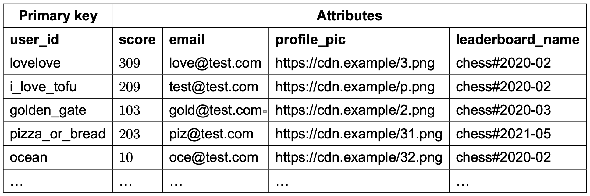
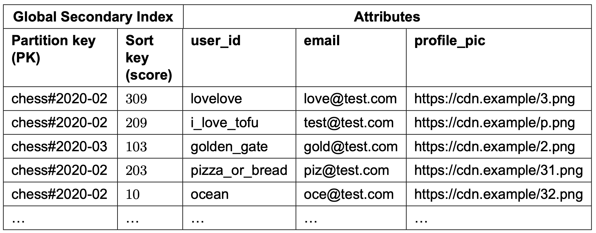
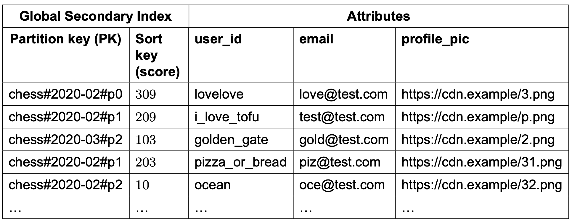
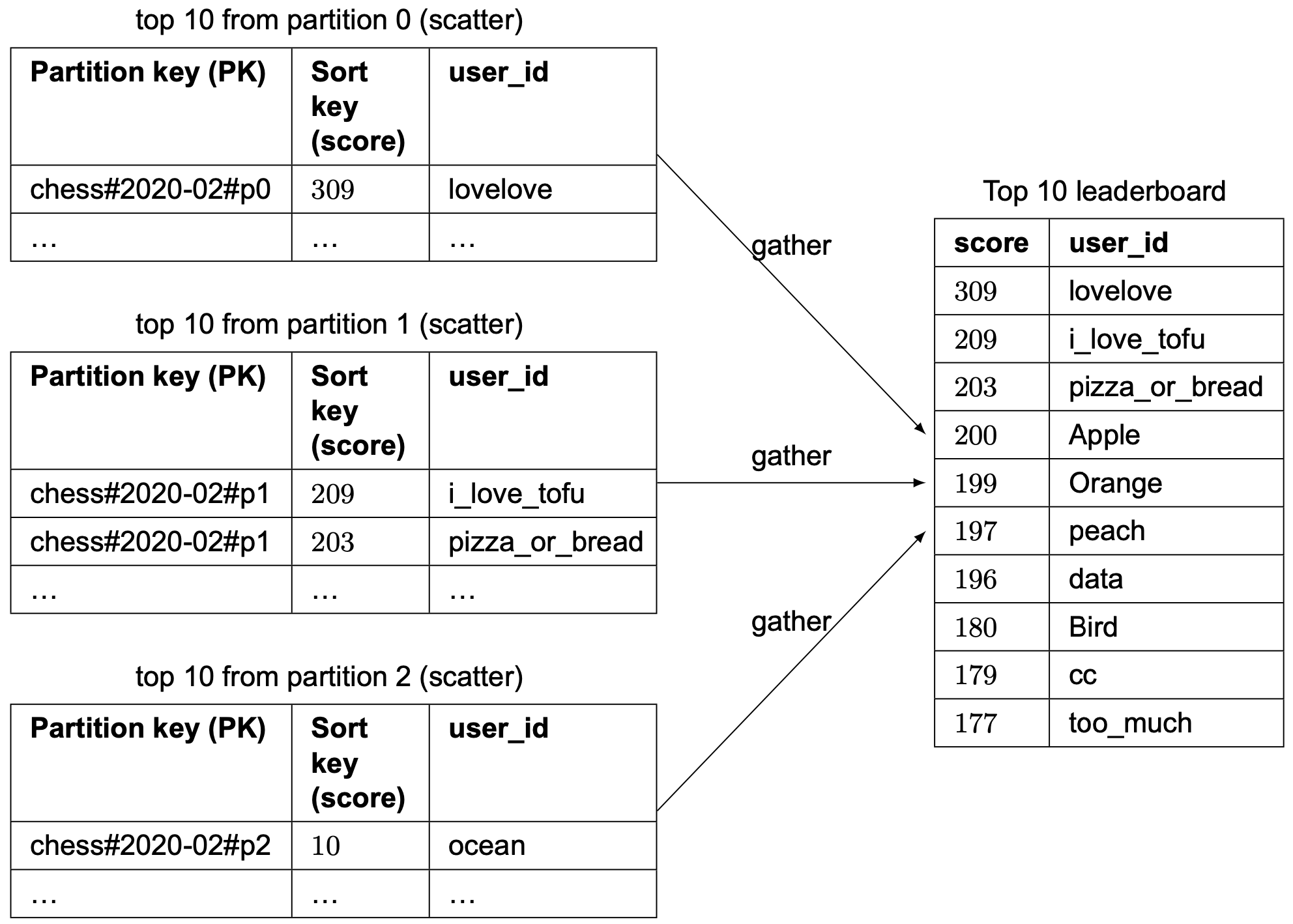
Step 4 - Wrap Up
Key design topics: Redis sorted sets with skip list internals (O(log n) operations), MySQL for persistence and recovery, Redis fixed partition sharding for 500M DAU scale, DynamoDB with write sharding as alternative.
**Additional talking points:** - **Tie-breaking:** Redis Hash stores `user_id → timestamp of last win`; earlier timestamp ranks higher when scores are equal. - **Failure recovery:** Replay MySQL win history through ZINCRBY calls to rebuild leaderboard from scratch.
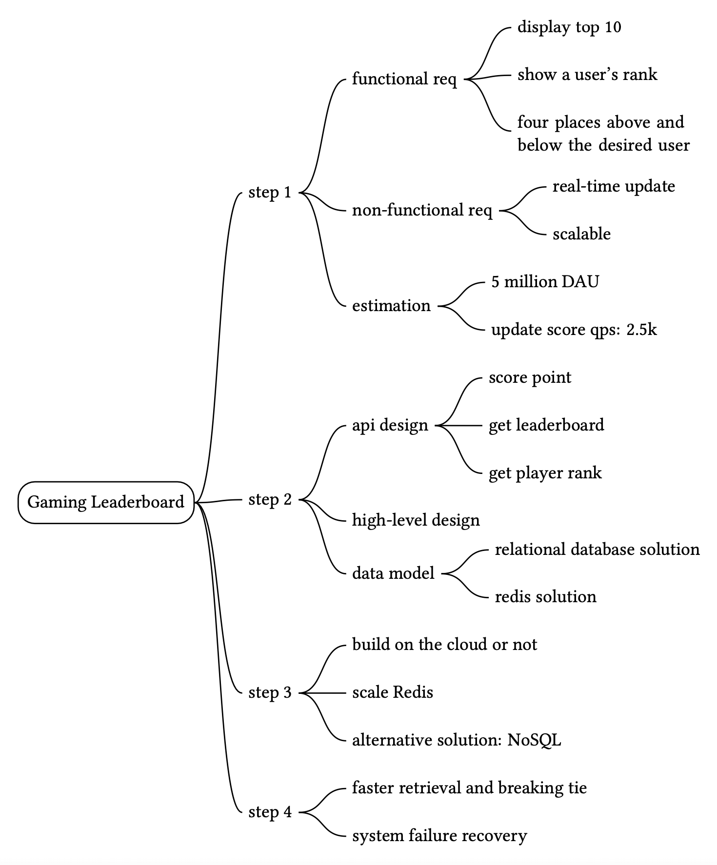
Payment System
We design a payment backend for an e-commerce application like Amazon. The payment system handles all money movement: collecting payments from buyers (pay-in) and disbursing funds to sellers (pay-out). Scale: 1 million transactions/day = ~10 TPS. Focus is on correctness, not throughput.
Step 1 - Understand the Problem and Establish Design Scope
**Functional requirements:** - **Pay-in flow** — Payment system receives money from customers on behalf of sellers. - **Pay-out flow** — Payment system sends money to sellers. - Credit card payment example (third-party PSPs like Stripe, Braintree, Square). - No card data stored internally (PCI DSS compliance via PSP). - Single currency for simplicity; global application.
**Non-functional requirements:** - Reliability and fault tolerance — failed payments carefully handled. - Reconciliation — async verification of payment consistency across internal and external services.
**Back-of-the-envelope:** 1M transactions/day ÷ 10⁵ seconds = **10 TPS**. Not a high-throughput problem — focus is on correctness.
Step 2 - Propose High-Level Design and Get Buy-In
**Pay-in vs Pay-out (Figure 1):** - Buyer pays → money goes to Amazon's bank account (pay-in). - Amazon acts as money custodian; seller owns most of the money. - After delivery, money flows from Amazon to seller's bank (pay-out).
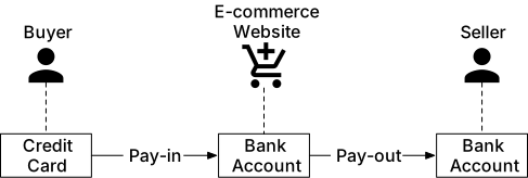
Pay-in flow
**Components (Figure 2):** - **Payment service** — Accepts payment events; runs risk check (AML/CFT via third-party); coordinates the process. - **Payment executor** — Executes a single payment order via PSP. One payment event can contain multiple orders (multi-seller checkout). - **PSP (Payment Service Provider)** — Moves money between accounts (e.g., Stripe, Braintree). Charges buyer's credit card. - **Card schemes** — Visa, MasterCard, Discovery. Process credit card operations. - **Ledger** — Immutable financial record using double-entry accounting. Used for revenue analysis and forecasting. - **Wallet** — Tracks merchant account balance and total user payments.
**Pay-in flow (9 steps):** 1. User clicks "place order" → payment event sent to payment service. 2. Payment service stores event in DB. 3. Payment event may contain multiple orders → payment service calls executor per order. 4. Payment executor stores order in DB. 5. Payment executor calls PSP to process credit card charge. 6. After success → payment service updates wallet (seller balance). 7. Wallet server stores updated balance. 8. Payment service calls ledger to record transaction. 9. Ledger appends new record.
**APIs:** - `POST /v1/payments` — Execute a payment event. Fields: `buyer_info`, `checkout_id`, `credit_card_info`, `payment_orders[]`. - Each payment order: `seller_account`, `amount` (string, not double — avoids floating point precision errors), `currency` (ISO 4217), `payment_order_id` (used as PSP idempotency key). - `GET /v1/payments/{:id}` — Get execution status of a payment order.
**Why amount as string (not double):** Floating point rounding errors across protocols/hardware; extreme values (Japan GDP in yen, Bitcoin satoshi = 10⁻⁸). Parse to number only for display/calculation.
**Data model:** - `payment_event` table: `checkout_id (PK)`, `buyer_info`, `seller_info`, `credit_card_info`, `is_payment_done`. - `payment_order` table: `payment_order_id (PK)`, `buyer_account`, `amount`, `currency`, `checkout_id (FK)`, `payment_order_status` (NOT_STARTED → EXECUTING → SUCCESS/FAILED), `ledger_updated`, `wallet_updated`.
**Database choice:** Traditional relational DB with ACID — stability over performance. Not NoSQL/NewSQL.
**Double-entry ledger:** Every transaction debits one account and credits another by the same amount. Sum of all entries = 0. Ensures end-to-end traceability.
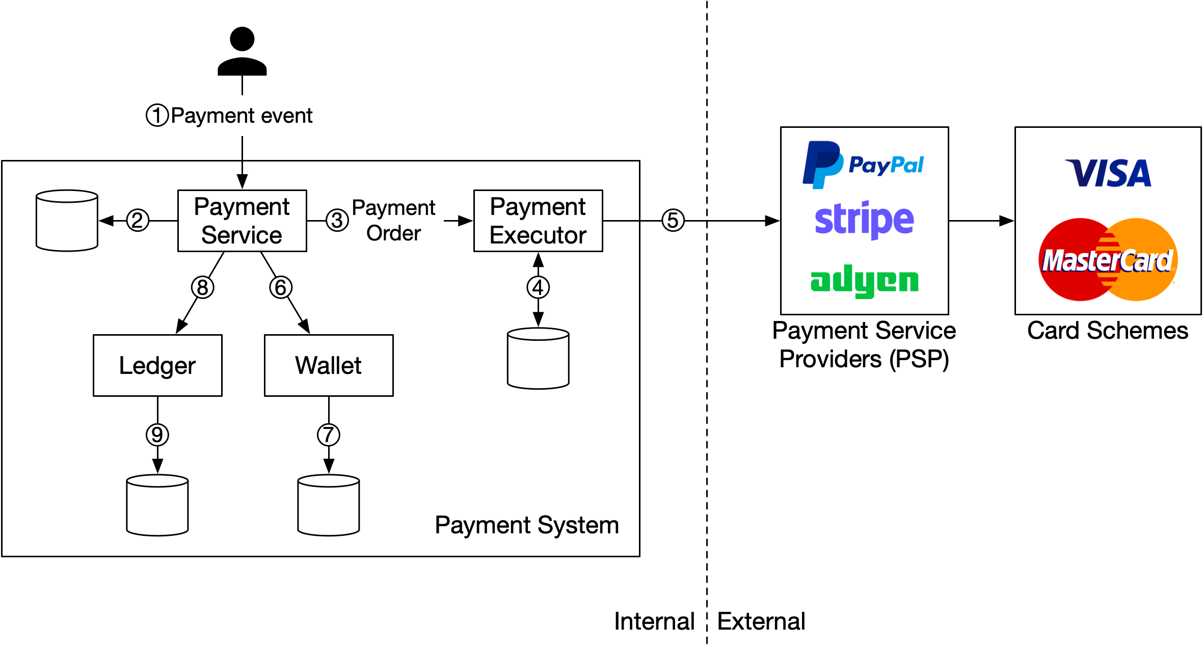
Hosted payment page (PSP integration)
Most companies use PSP-hosted payment pages (iframe/widget/SDK) to avoid storing card data and PCI DSS liability.
**Example: PayPal integration (Figure 3)** — PSP shows its own UI for card capture.
**9-step hosted payment flow (Figure 4):** 1. User clicks checkout → client calls payment service with order info. 2. Payment service sends registration request to PSP with amount, currency, expiration, redirect URL, and **nonce** (UUID idempotency key = payment_order_id). Ensures exactly-once registration. 3. PSP returns **token** (UUID identifying this payment registration). 4. Payment service stores token in DB. 5. Client displays PSP-hosted payment page (Figure 5 — Stripe example). PSP JS library collects card info directly; card data never touches our system. - PSP JS uses token to retrieve payment details from PSP backend. - Redirect URL specified for post-payment navigation. 6. User fills card details → clicks pay → PSP starts processing. 7. PSP returns payment status. 8. Browser redirected to redirect URL (payment status appended to URL). 9. Asynchronously, PSP calls our registered **webhook** with payment status → payment service updates `payment_order_status`.
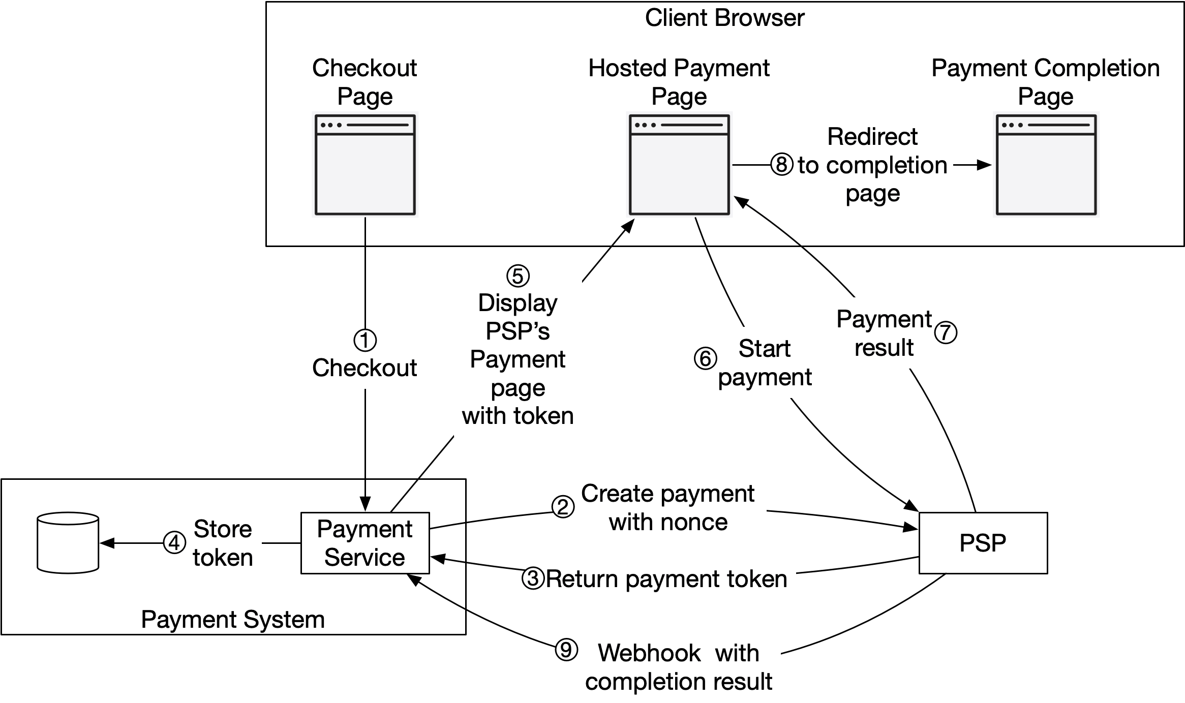
Pay-out flow
Similar to pay-in but in reverse direction. Uses third-party **pay-out providers** (e.g., Tipalti) to move money from e-commerce site's bank account to sellers' bank accounts. Complex regulatory and bookkeeping requirements apply.
Step 3 - Design Deep Dive
Reconciliation
**The last line of defense** for payment correctness. Async verification that states across services are consistent.
**Process (Figure 6):** Every night, PSPs/banks send **settlement files** containing all transactions and account balance for the day. Reconciliation system parses the file and compares with the internal ledger.
**Three types of mismatches:** 1. **Classifiable + auto-fixable** — Known cause with automated adjustment. 2. **Classifiable but manual** — Known cause, too complex to automate. Goes into job queue for finance team. 3. **Unclassifiable** — Unknown cause. Special queue for manual investigation by finance team.
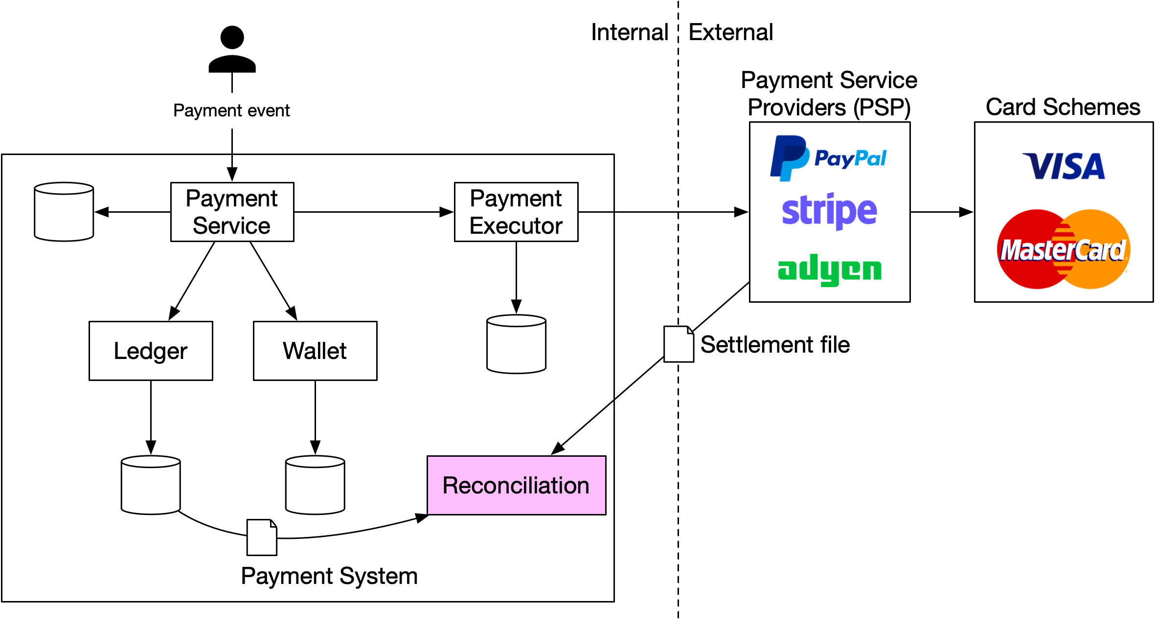
Handling payment processing delays
Some payment requests take hours or days (high-risk flagged for human review, 3D Secure authentication required).
**PSP handling:** - Returns **pending status** to client; client shows pending state. - PSP tracks pending payment and notifies payment service via webhook when resolved.
**Alternative:** Some PSPs require payment service to poll for status updates.
Communication among internal services
**Synchronous (HTTP):** Simple but creates tight coupling. Drawbacks: low performance, poor failure isolation, hard to scale.
**Asynchronous messaging:** - **Single receiver (Figure 7-8):** Each message processed by one consumer; message removed after processing. Standard message queue (e.g., SQS). - **Multiple receivers (Figure 9):** Same message consumed by many services. Kafka retains messages. Maps well to payment system: score update triggers payment processing + analytics + billing + push notifications simultaneously.
**Recommendation:** Asynchronous for large-scale payment systems — better scalability and failure resilience despite added complexity.
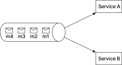
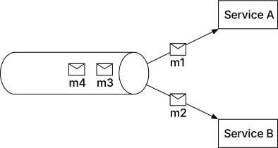
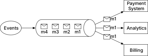
Handling failed payments
**Payment state tracking:** Payment state persisted in append-only table at every stage. On failure, current state determines whether to retry or refund.
**Retry queue + dead letter queue (Figure 10):** 1. Failure occurs → check if retryable. - 1a. Retryable (transient errors) → retry queue. - 1b. Non-retryable (invalid input) → stored in DB. 2. Payment system consumes from retry queue and retries. 3. If fails again: - 3a. Retry count under threshold → back to retry queue. - 3b. Retry count exceeds threshold → **dead letter queue** (for debugging and manual investigation).
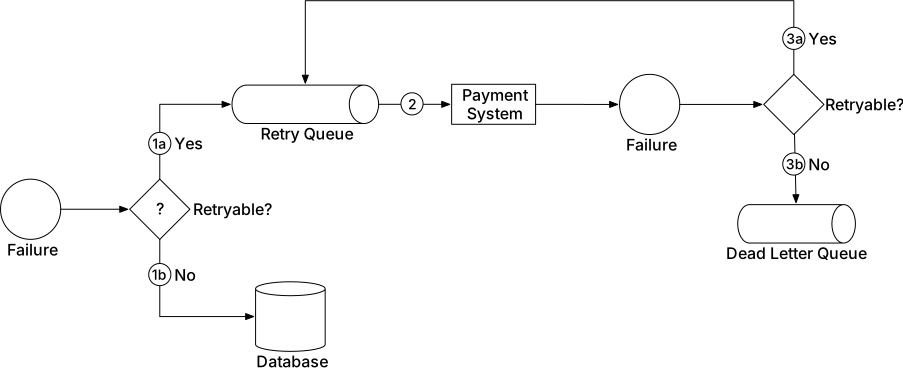
Exactly-once delivery
**Exactly-once = at-least-once (retry) AND at-most-once (idempotency)**.
**Retry — at-least-once guarantee (Figure 11):** Strategies (worst to best for network issues): - Immediate retry — can worsen congestion. - Fixed intervals. - Incremental intervals. - **Exponential backoff** — doubles wait time (1s → 2s → 4s). Best for transient network issues. - Cancel — for permanent failures.
Provide `Retry-After` header with error codes.
**Idempotency — at-most-once guarantee (Figure 12):** - Client generates idempotency key (UUID, e.g., shopping cart ID) in HTTP header: `idempotency-key: <value>`. - Server uses DB unique key constraint: first insert succeeds; duplicate insert fails → return cached response. - Concurrent requests with same key → one processed, others receive 429 Too Many Requests.
**Scenario 1 (double-click):** Idempotency key prevents second charge.
**Scenario 2 (network error, user re-submits):** PSP token uniquely maps to payment order. Same order → same token → PSP identifies it as duplicate → returns previous execution status.
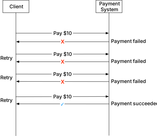
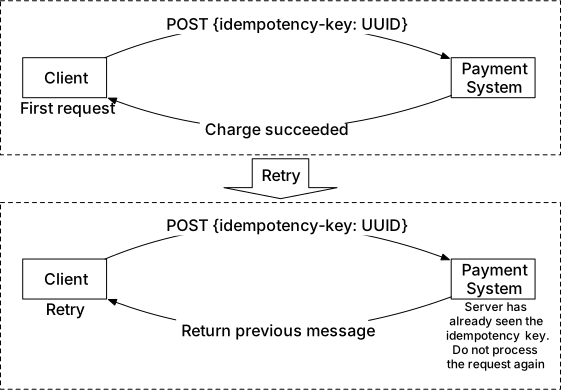
Consistency
Stateful services involved: payment service, ledger, wallet, PSP, DB replicas.
**Internal consistency:** Exactly-once processing prevents divergence between services.
**External consistency (with PSP):** Use same idempotency key for retries. Even if PSP supports idempotency, still run reconciliation — don't assume external system is always correct.
**Replication lag options:** 1. Read + write from primary only — simple but wastes replica resources. 2. Keep replicas always in-sync — use Paxos/Raft consensus, or consensus-based DB (YugabyteDB, CockroachDB).
Payment security
| Problem | Solution | |---------|----------| | Request/response eavesdropping | HTTPS | | Data tampering | Encryption + integrity monitoring | | Man-in-the-middle attack | SSL with certificate pinning | | Data loss | DB replication + snapshots | | DDoS | Rate limiting + firewall | | Card theft | Tokenization (store tokens, not card numbers) | | PCI compliance | PCI DSS standard | | Fraud | Address verification, CVV, user behavior analysis |
Step 4 - Wrap Up
Key design topics: pay-in/pay-out flows, hosted PSP payment page with nonce/token/webhook, double-entry ledger, reconciliation with settlement files, retry queues + dead letter queues, exactly-once delivery via retry + idempotency, payment security.
Additional topics: monitoring/alerting, debugging tools, currency exchange, geography-specific payment methods, cash payments, Google/Apple Pay integration.
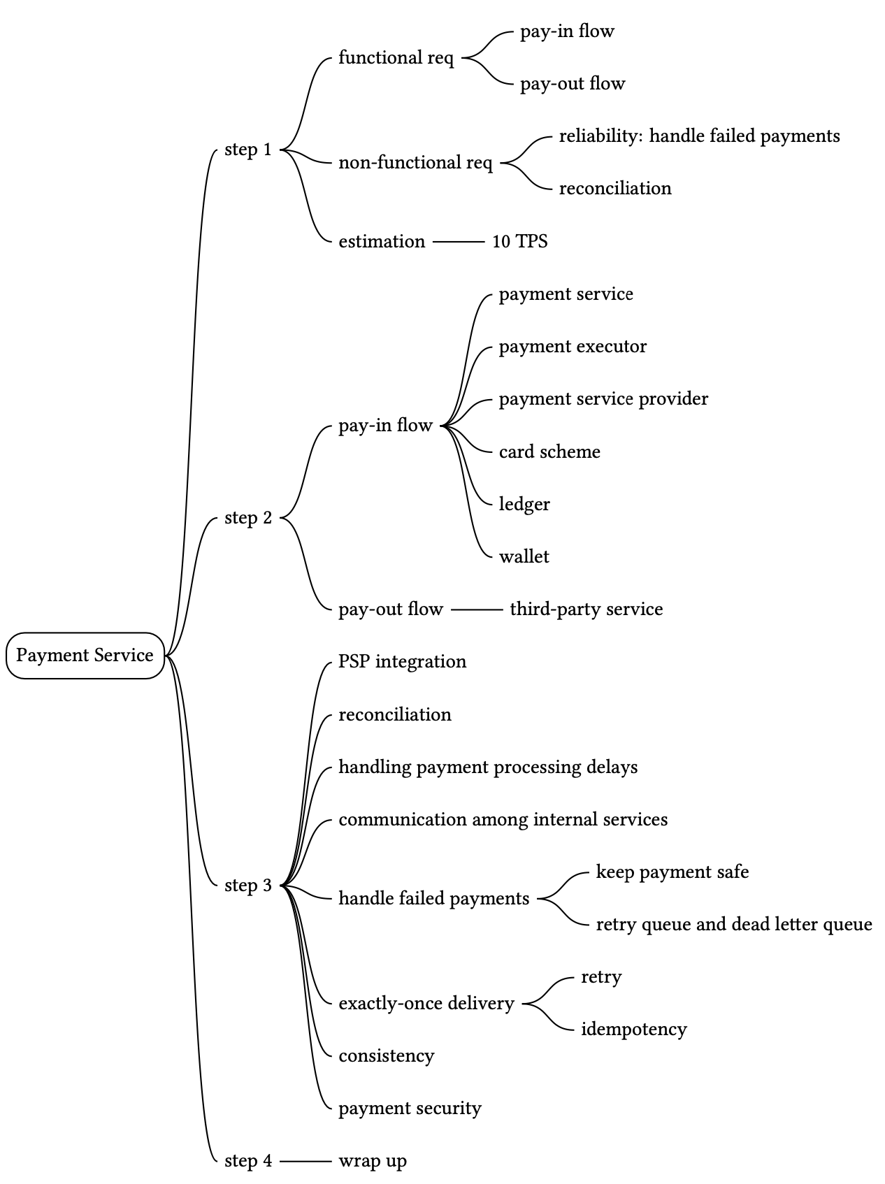
Digital Wallet
Payment platforms provide a digital wallet service: users store money and spend it later, or transfer directly to another wallet on the same platform (faster and usually free vs bank-to-bank transfers). We design the backend supporting cross-wallet balance transfers at 1M TPS with transactional guarantees and reproducibility.

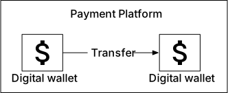
Step 1 - Understand the Problem and Establish Design Scope
**Requirements:** - Balance transfer between two digital wallets only. - **1,000,000 TPS**. - Reliability ≥ 99.99%. - Transactional guarantees. - **Reproducibility** — reconstruct historical balance by replaying data from the beginning (not just reconciliation, which only shows discrepancies). - No foreign exchange (out of scope).
Back-of-the-envelope estimation
Each transfer = 2 DB operations (deduct + deposit). At 1M transfers/sec → **2M TPS**.
| Per-node TPS | Node Number | |-------------|-------------| | 100 | 20,000 | | 1,000 | 2,000 | | 10,000 | 200 |
Design goal: maximize per-node TPS to reduce hardware cost.
Step 2 - Propose High-Level Design and Get Buy-In
Three high-level designs explored: 1. Simple in-memory solution (Redis) 2. Database-based distributed transaction solution (2PC, TC/C, Saga) 3. Event sourcing solution with reproducibility
API Design
Single REST endpoint:
| API | Detail | |-----|--------| | `POST /v1/wallet/balance_transfer` | Transfer balance from one wallet to another |
**Request parameters:**
| Field | Description | Type | |-------|-------------|------| | `from_account` | Debit account | string | | `to_account` | Credit account | string | | `amount` | Amount (string, not double — avoids floating point precision errors) | string | | `currency` | ISO 4217 | string | | `transaction_id` | UUID for deduplication/idempotency | uuid |
**Response:** `{ "Status": "success", "Transaction_id": "..." }`
In-memory sharding solution
Use a cluster of Redis nodes to store `{user → balance}` map. Shard by `accountID.hashCode() % N`. Zookeeper stores sharding configuration. Stateless wallet service looks up partition and updates two Redis nodes per transfer.
**Problem:** No atomicity across two Redis nodes. If wallet service crashes after updating node A but before node B, the transfer is incomplete. Two updates must be in a single atomic transaction.
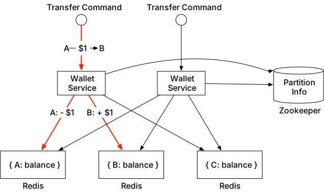
Distributed transactions
Replace Redis with transactional relational databases to enable atomicity per node. Still need coordination across nodes for a single transfer.
Database sharding
Partition accounts across multiple relational DB nodes (instead of Redis). Each DB node provides local ACID guarantees, but a transfer spanning two nodes still requires distributed coordination.
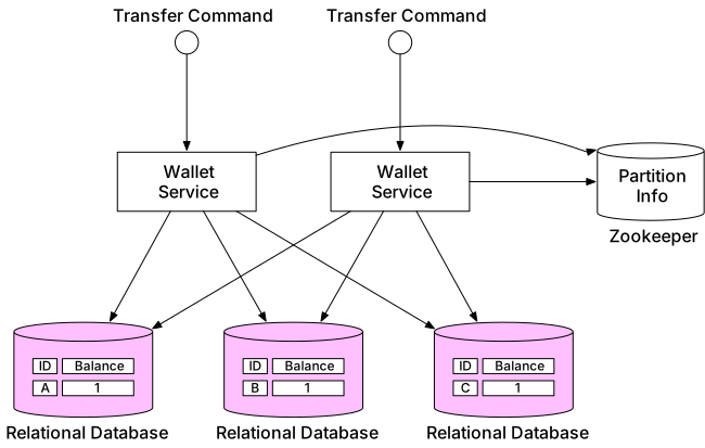
Distributed transaction: two-phase commit (2PC)
Low-level solution relying on DB support (e.g., X/Open XA standard).
**Two phases:** 1. Coordinator (wallet service) performs read/write on multiple DBs — **both are locked**. 2. Coordinator asks all DBs to prepare: - All reply "yes" → coordinator commits all. - Any reply "no" → coordinator aborts all.
**Problems:** - **Performance**: Locks held for a long time waiting for messages from other nodes. - **SPOF**: Coordinator is a single point of failure — if it crashes after phase 1, locks are held indefinitely.
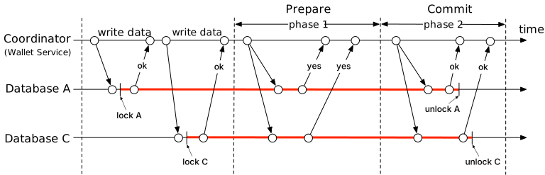
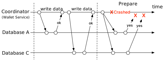
Distributed transaction: Try-Confirm/Cancel (TC/C)
High-level compensating transaction. Unlike 2PC, each phase is an **independent local transaction** (no long-held locks).
**Phases:** 1. **Try** — coordinator asks all DBs to reserve resources. 2. **Confirm** (if all say yes) — execute the actual operations. 2. **Cancel** (if any say no) — undo the Try phase effects (compensating transactions).
**Example: Transfer $1 from A to C:**
| Phase | Operation | A | C | |-------|-----------|---|---| | 1 | Try | -$1 | NOP | | 2 | Confirm | NOP | +$1 | | | Cancel | +$1 (undo) | NOP |
**Why only Choice 1 is valid for Try phase:** - Choice 2 (NOP on A, +$1 on C): C might get spent before the Cancel can reverse it. - Choice 3 (-$1 A and +$1 C simultaneously): Complex failure cases.
**Unbalanced state:** During Try, $1 is deducted from A but C not yet credited — sum is temporarily less. This intermediate inconsistency is visible to the application (unlike 2PC/DB transactions which hide it).
**Phase status table:** Stored in A's database. Tracks: distributed transaction ID/content, Try phase status per DB (not sent / sent / response received), second phase name (Confirm or Cancel), second phase status, out-of-order flag. Enables crash recovery.
**Out-of-order execution:** Cancel may arrive at C before Try (due to network issues). Solution: Cancel leaves an out-of-order flag; subsequent Try detects flag and returns failure.
**vs 2PC:**
| | First Phase | Second Phase: success | Second Phase: fail | |--|-------------|----------------------|--------------------| | 2PC | Local transactions not done yet (locked) | Commit all | Cancel all | | TC/C | All local transactions completed | Execute new local transactions if needed | Reverse ("undo") committed transactions |
TC/C is database-agnostic (works with any DB supporting transactions) but complexity is in application business logic.
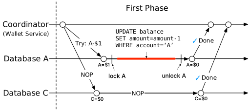
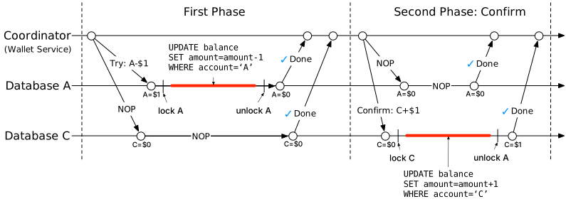
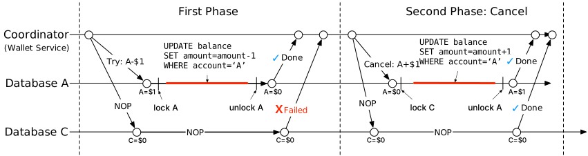
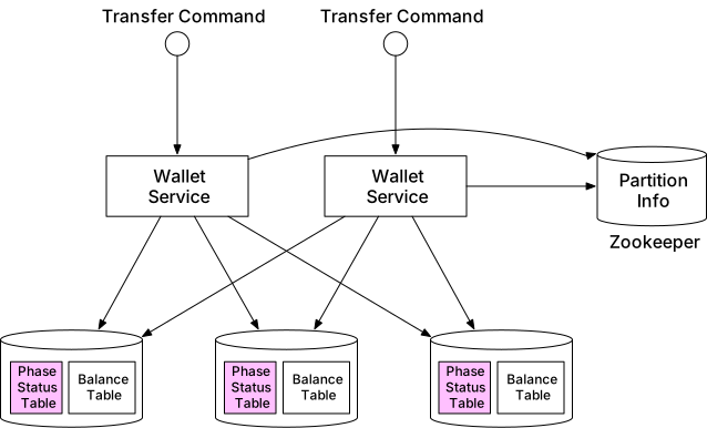
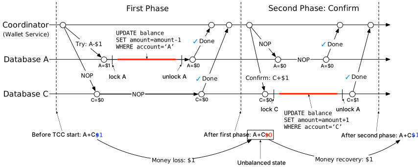
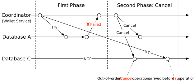
Distributed transaction: Saga
De-facto standard in microservice architecture.
**Rules:** - Operations ordered in a **linear sequence**; each is an independent DB transaction. - Operations execute one by one; completion triggers the next. - On failure: **rollback** from current operation to first, using compensating transactions. - `n` operations → `2n` total (n forward + n compensating).
**Coordination modes:** - **Choreography** — services subscribe to each other's events (fully decentralized). Hard to manage with many services — each must maintain an internal state machine. - **Orchestration** — single coordinator directs all services in order. Handles complexity well; preferred for digital wallets.
**vs TC/C:**
| | TC/C | Saga | |--|------|------| | Compensating action | Cancel phase | Rollback phase | | Central coordination | Yes | Yes (orchestration) | | Operation execution order | Any | Linear only | | Parallel execution | Yes | No | | Partial inconsistency visible | Yes | Yes |
**When to choose:** Latency-sensitive + many services → TC/C (parallel). Fewer services / microservice trend → Saga.
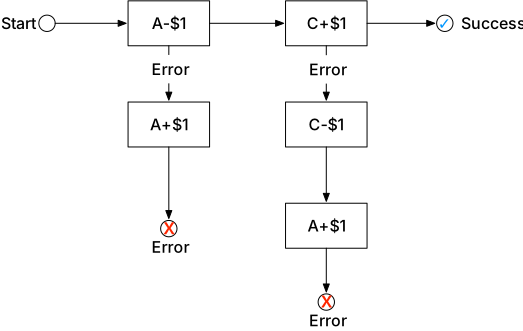
Event sourcing
Chosen for auditability and reproducibility — answers auditor questions: - Account balance at any given time? (replay events up to that point) - How to verify historical balances are correct? (recalculate from event list) - How to prove logic is correct after code change? (run different versions against same events)
Background
Distributed transaction solutions only save updated state — you cannot audit *why* a balance changed. Event sourcing stores all changes as immutable history; state is a derived view, always reconstructable.
Definition
Four core concepts:
**Command** — intended action from the outside world (e.g., "transfer $1 from A to C"). Commands are put in a FIFO queue. May be invalid.
**Event** — validated, fulfilled command result (past tense: "transferred $1 from A to C"). Must be executed. **Deterministic** — no randomness or I/O. Events are stored in a FIFO queue. One command → 0 or more events (event generation may contain randomness; events themselves must be deterministic).
**State** — what changes when an event is applied. In the wallet system: `{account → balance}` map. Stored in a key-value store or relational DB.
**State machine** — drives event sourcing: 1. Validates commands and generates events. 2. Applies events to update state. Must be **fully deterministic** — no external I/O, no random numbers. Same events always produce same state.
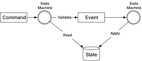
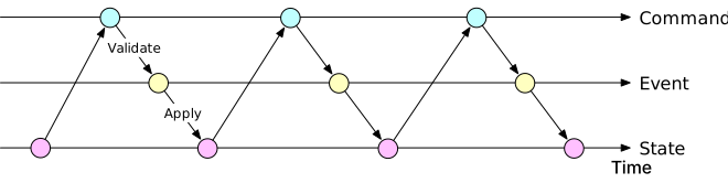
Wallet service example
Commands = balance transfer requests → Kafka FIFO queue. State = account balances in relational DB.
**State machine (5 steps):** 1. Read command from command queue. 2. Read balance state from DB. 3. Validate command; if valid, generate two events (e.g., `A:-$1`, `C:+$1`). 4. Read next event. 5. Apply event — update balance in DB.
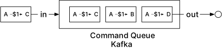
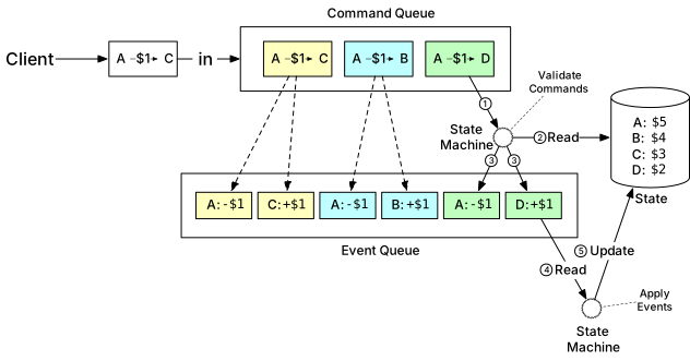
Reproducibility
Event list is **immutable**. State machine is **deterministic**. Therefore: replaying events from the beginning always regenerates the same historical states.
Distributed transaction solutions lose history on state update. Event sourcing keeps all history; DB is just a current-view cache of the event log.
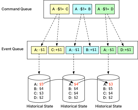
Command-query responsibility segregation (CQRS)
External clients need to query current balance — but event sourcing's internal state isn't directly exposed.
**CQRS pattern:** Rather than publishing state, publish all events. External consumers rebuild their own customized state views.
- **One write state machine** — maintains authoritative event log. - **Many read-only state machines** — subscribe to event queue, build materialized views for different query needs (current balances, time-range audits, double-charge investigation, reconciliation).
Read-only state machines lag behind but always catch up → **eventually consistent**.
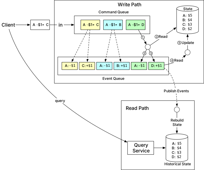
Step 3 - Design Deep Dive
Deep dive into high performance, reliability, and scalability for the event sourcing architecture.
High-performance event sourcing
Move from remote Kafka + remote DB to local file-based storage to eliminate network latency.
File-based command and event list
**Optimization 1:** Save commands and events to **local disk** (not remote Kafka) — eliminates network round-trips. Uses append-only structure (sequential writes, OS-optimized; can be faster than random memory access).
**Optimization 2:** Cache recent commands/events in **memory** — skip disk reads for recently written data.
**Implementation:** Use `mmap` — maps a disk file to a memory array. OS caches hot sections in memory. For append-only operations: data is nearly always in memory cache.
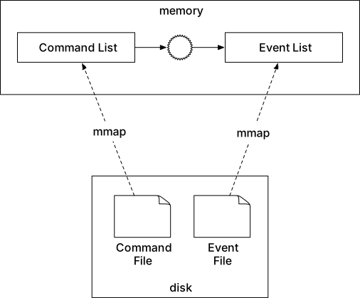
File-based state
Move state from remote relational DB to local file-based stores: - **SQLite** — file-based local relational DB. - **RocksDB** — file-based key-value store using LSM tree (optimized for writes; caches recent data for reads). Preferred choice.
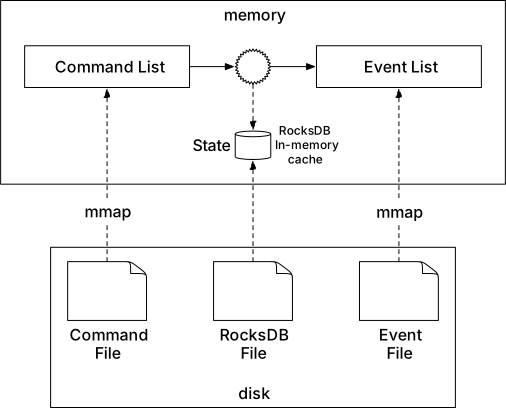
Snapshot
**Problem:** Reproducibility requires replaying from event #1 every time.
**Solution:** Periodically stop the state machine and save current state to a **snapshot file** (immutable historical state view). On restart/replay: load nearest snapshot, verify position, resume from there.
Finance teams often require snapshots at 00:00 to verify daily transactions. Read-only state machines load one snapshot instead of replaying all events from genesis.
Snapshot files are large binary files — stored in object storage (e.g., HDFS).
With everything file-based, the system can fully utilize maximum I/O throughput of local hardware.
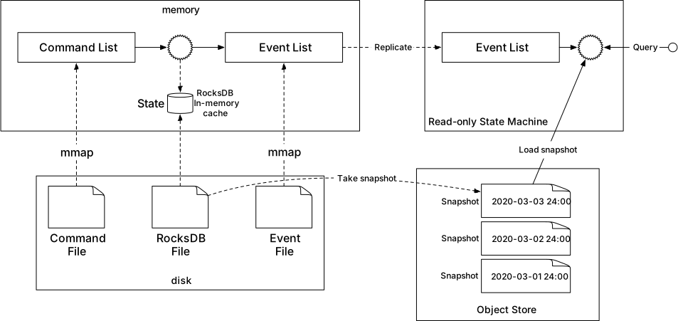
Reliable high-performance event sourcing
File-based local storage creates a single point of failure. Need replication.
Reliability analysis
**Four data types:** 1. File-based command 2. File-based event 3. File-based state 4. State snapshot
**Analysis:** - State and snapshot can always be regenerated from the event list → just protect events. - Command cannot guarantee event reproducibility (event generation may be non-deterministic — contains external I/O, random numbers). - **Event** is the only data requiring strong reliability guarantee. Events are deterministic facts; replaying them always reconstructs the same state.
**Conclusion: Only the event list needs high-reliability replication.**
Consensus
Use **Raft consensus algorithm** to replicate event list across multiple nodes.
**Guarantees:** As long as majority of nodes are online, all append-only event lists have the same data.
**Raft node roles:** Leader, Candidate, Follower. - At most one leader per cluster. - Leader receives commands, replicates events reliably. - **3 nodes** → tolerates 1 failure. **5 nodes** → tolerates 2 failures.

Reliable solution
**3-node event sourcing cluster with Raft (Figure 24):** - Leader accepts incoming commands, converts to events, appends to local event list. - Raft replicates new events to followers. - All nodes (leader + followers) process event list and update state → identical states guaranteed.
**Failure handling:** - **Leader crash:** Raft auto-elects new leader. Client resends command (crash may have occurred before command→event conversion). Idempotency key (transaction_id) prevents double processing. - **Follower crash:** Raft retries indefinitely until node restarts or is replaced.
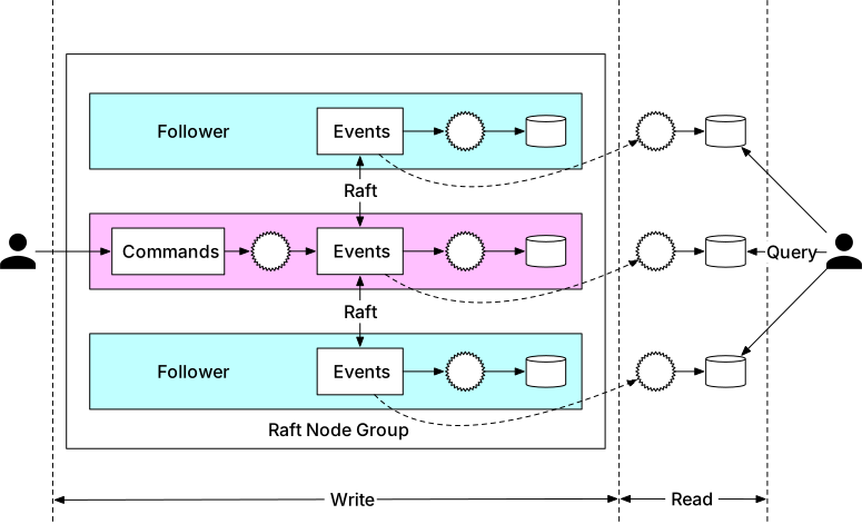
Distributed event sourcing
Single Raft group has two limitations: 1. CQRS response is slow — client must poll for execution status. 2. Capacity of one Raft group is limited — need sharding + distributed transactions at scale.
Pull vs push
**Pull model (Figure 25):** External user polls read-only state machine periodically. Not real-time; can overload wallet service.
**Pull + reverse proxy (Figure 26):** User sends command to reverse proxy, which polls on user's behalf. Simplifies client logic but still not real-time.
**Push model (Figure 27):** Read-only state machine pushes execution status back to reverse proxy as soon as event is received. User gets near real-time response.
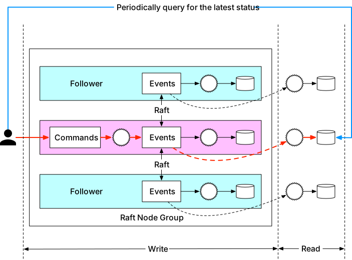
Distributed transaction
With push model making each Raft group synchronous, reuse TC/C or Saga for cross-partition coordination.
**Partition scheme:** Hash key by 2 → Partition 1 (account A) and Partition 2 (account C).
**Final distributed event sourcing design (Figure 28):** Saga coordinator + multiple Raft partition groups.
**29-step Saga happy path (Figure 29): Transfer $1 from A to C:** 1. User A sends distributed transaction to Saga coordinator (A-$1, C+$1). 2. Saga coordinator creates record in phase status table. 3. Coordinator sends A-$1 command to Partition 1. 4. Partition 1 Raft leader stores command, validates, converts to event, Raft synchronizes across nodes, executes (deduct $1 from A). 5. Partition 1 CQRS synchronizes to read path; read path reconstructs state and execution status. 6. Read path of Partition 1 pushes status to Saga coordinator. 7. Saga coordinator receives success from Partition 1. 8. Coordinator records Partition 1 success in phase status table. 9. Coordinator sends C+$1 command to Partition 2. 10. Partition 2 Raft leader stores command, validates, converts to event, Raft synchronizes, executes (add $1 to C). 11. Partition 2 CQRS synchronizes to read path; reconstructs state. 12. Read path of Partition 2 pushes status to Saga coordinator. 13. Saga coordinator receives success from Partition 2. 14. Coordinator records Partition 2 success in phase status table. 15. All operations complete; coordinator responds to caller with success.
Step 4 - Wrap Up
**Evolution of designs:** 1. **In-memory Redis sharding** — fast but no atomicity across nodes. 2. **Distributed transactions (2PC / TC/C / Saga)** — atomicity achieved but no audit trail. 3. **Event sourcing (remote Kafka + DB)** — reproducibility but slow (network). 4. **File-based event sourcing** — high performance via local mmap + RocksDB. 5. **Raft replication** — eliminates single point of failure. 6. **CQRS + reverse proxy (push)** — synchronous response for external users. 7. **Saga across Raft partition groups** — final scalable, reliable, auditable design.
**Key properties achieved:** 1M+ TPS, transactional guarantees, 99.99% reliability, full reproducibility for audits.
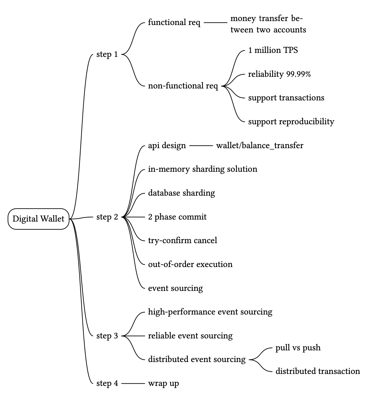
Stock Exchange
We design an electronic stock exchange system. The basic function is to efficiently match buyers and sellers. Today orders are processed by supercomputers at NYSE (billions of matches/day) and HKEX (~200 billion shares/day). Scale matters — check with the interviewer for size and characteristics.
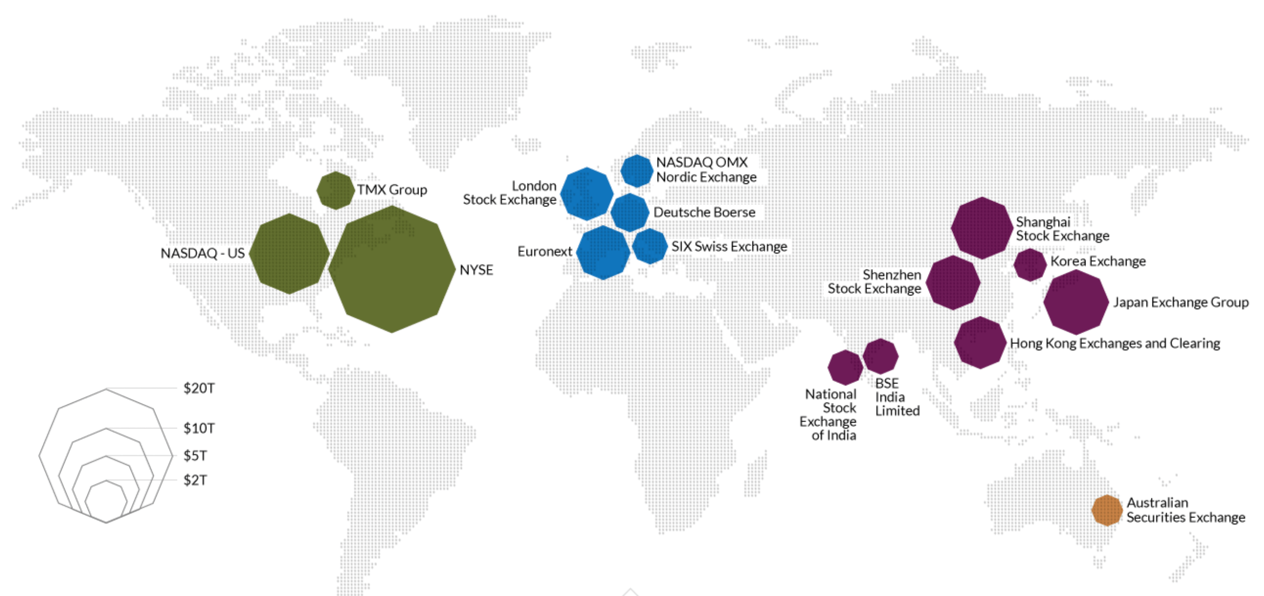
Step 1 - Understand the Problem and Establish Design Scope
**Functional requirements:** - Securities: **stocks only** (no options/futures). - Operations: **place** and **cancel** limit orders. - Order types: **limit orders only** (no market or conditional orders). - Trading hours: normal hours only (no after-hours). - Support tens of thousands of concurrent users, ≥100 symbols, **billions of orders/day**. - Real-time order book (list of buy/sell orders) visible to clients. - **Risk checks** (e.g., max 1M shares of a single stock per user per day). - **Wallet management**: sufficient funds required; funds withheld for open orders.
Non-functional requirements
- **Availability**: ≥99.99%. - **Fault tolerance**: fast recovery mechanism to limit production incident impact. - **Latency**: millisecond-level round-trip (order enters exchange → filled execution returned). Focus on **99th percentile** latency. - **Security**: KYC (Know Your Client) for new accounts; DDoS protection for public endpoints.
Back-of-the-envelope estimation
- 100 symbols, 1 billion orders/day. - NYSE open 6.5 hours/day (9:30am–4:00pm ET). - **QPS**: 1B / 6.5 / 3600 ≈ **43,000**. - **Peak QPS**: 5× = **215,000** (high volume at market open/close).
Step 2 - Propose High-Level Design and Get Buy-In
Key concepts: brokers (Charles Schwab, Robinhood), institutional clients (pension funds, hedge funds/market makers), limit orders, market orders, market data levels, candlestick charts, FIX protocol.
Business Knowledge 101
**Broker** — retail clients trade via brokers (web/mobile UI). Institutional clients use specialized software.
**Limit order** — fixed price buy/sell; may not match immediately or may be partially filled.
**Market order** — no price specified; executed at prevailing price immediately; sacrifices cost for guaranteed execution.
**Market data levels:** - **L1** — best bid price, ask price, quantities (Figure 2). - **L2** — more price levels than L1 (Figure 3). - **L3** — price levels with queued quantity at each level (Figure 4).
**Candlestick chart** — shows open, close, high, low price for a time interval (1min, 5min, 1hr, 1day, 1week, 1month). Figure 5 shows a single candlestick.
**FIX protocol** — Financial Information eXchange (1991), vendor-neutral protocol for securities transactions.
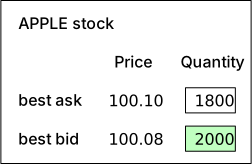
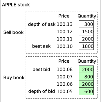
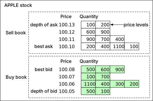
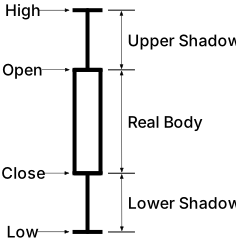
High-level design
Three flows (Figure 6):
**Trading flow (critical path, strict latency):** 1. Client places order via broker app. 2. Broker sends order to exchange. 3. Client gateway: input validation, rate limiting, authentication, normalization → forward to order manager. 4–5. Order manager performs risk checks. 6. Order manager verifies sufficient wallet funds. 7–9. Order sent to matching engine via sequencer (stamped with sequence ID); match produces two executions (fills) for buy/sell sides; outbound sequencer stamps executions. 10–14. Executions returned to client via client gateway.
**Market data flow (non-critical):** - M1: Matching engine generates execution stream → market data publisher (MDP). - M2: MDP builds candlestick charts and order books → data service. - M3: Market data saved to specialized storage; brokers relay to clients.
**Reporting flow (non-critical):** - R1–R2: Reporter collects order + execution fields (client_id, price, quantity, order_type, filled_quantity, remaining_quantity) → writes to database.
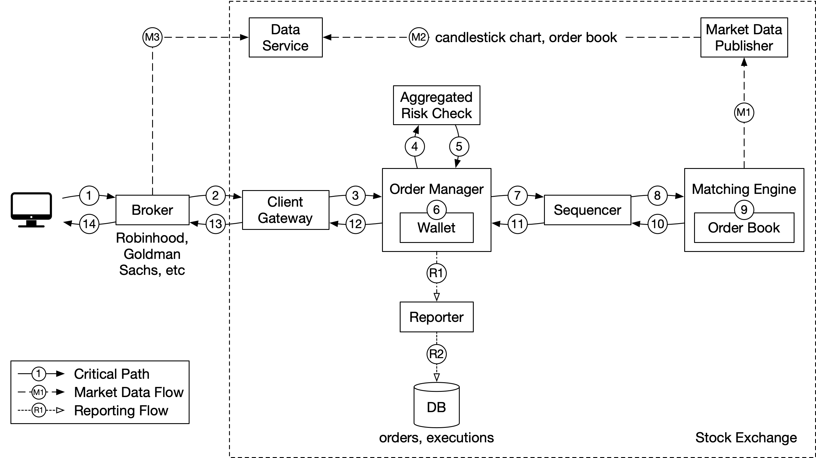
Trading flow
**Matching engine** (also called cross engine): - Maintains order book per symbol. - Matches buy/sell orders → two executions per match (buy side + sell side). - Distributes execution stream as market data. - Must be **deterministic**: given same input sequence → same output sequence (enables replay for HA).
**Sequencer** — makes matching engine deterministic (Figure 7): - **Inbound sequencer**: stamps incoming orders with sequential IDs before matching engine processes them. - **Outbound sequencer**: stamps outgoing executions with sequential IDs. - Sequential IDs → missing numbers easily detected. - Functions as: message queue, event store, exactly-once guarantee, fast replay. - Like two Kafka streams but lower and more predictable latency.
**Order manager**: - Receives inbound orders from client gateway. - Sends to risk check (e.g., user trade volume < $1M/day). - Verifies wallet has sufficient funds. - Sends order to sequencer (only necessary attributes, not all). - Receives executions from sequencer → returns to brokers. - Uses **event sourcing** for state management (handles many state transition cases).
**Client gateway** (Figure 8 & 9): - Gatekeeper: input validation, rate limiting, auth, normalization. - Stays lightweight — passes orders to destinations as fast as possible. - Different gateways for retail vs institutional (latency, volume, security). - **Colocation (colo)**: exchange trading software running on broker's server in exchange's data center; latency = speed of light between servers.
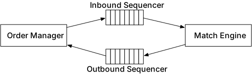
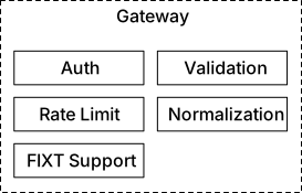
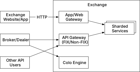
Market data flow
Market data publisher (MDP) receives executions from matching engine → builds order books and candlestick charts (collectively: market data) → sends to data service for subscribers.
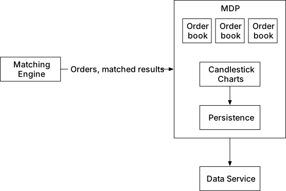
Reporting flow
Reporter is not on critical path but critical for the business: trading history, tax reporting, compliance, settlements. - Merges attributes from incoming orders + outgoing executions. - Less latency-sensitive; **accuracy and compliance** are key.
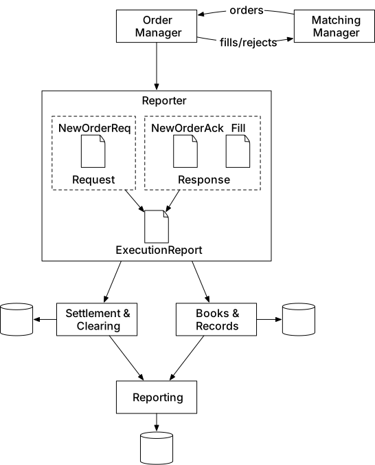
API Design
REST API between brokers and client gateway (institutional clients may use specialized lower-latency protocols).
**Place order:** `POST /v1/order` - Parameters: `symbol` (string), `side` (buy/sell), `price` (Long), `orderType` (limit/market), `quantity` (Long). - Response: `id`, `creationTime`, `filledQuantity`, `remainingQuantity`, `status` (new/canceled/filled).
**Get executions:** `GET /execution?symbol={}&orderId={}&startTime={}&endTime={}` - Response: array of executions with `id`, `orderId`, `symbol`, `side`, `price`, `orderType`, `quantity`.
**Order book:** `GET /marketdata/orderBook/L2?symbol={}&depth={}` - Response: `bids` and `asks` arrays (price + size).
**Candlestick charts:** `GET /marketdata/candles?symbol={}&resolution={}&startTime={}&endTime={}` - Response: `candles` array with `open`, `close`, `high`, `low` per interval.
Data models
Three main data types: product/order/execution, order book, candlestick chart.
Product, order, execution
- **Product** — symbol attributes (type, trading symbol, display symbol, currency, lot size, tick size). Rarely changes; highly cacheable. - **Order** — inbound buy/sell instruction. - **Execution (fill)** — outbound matched result. Matching engine produces two executions per match (buy + sell sides). Not every order has an execution.
**Storage:** - Critical trading path: in-memory + disk/shared memory (not DB). Stored in sequencer for fast recovery; archived after market closes. - Reporter: writes to DB for reconciliation/tax reporting. - MDP: uses executions to reconstruct order book and candlestick data.
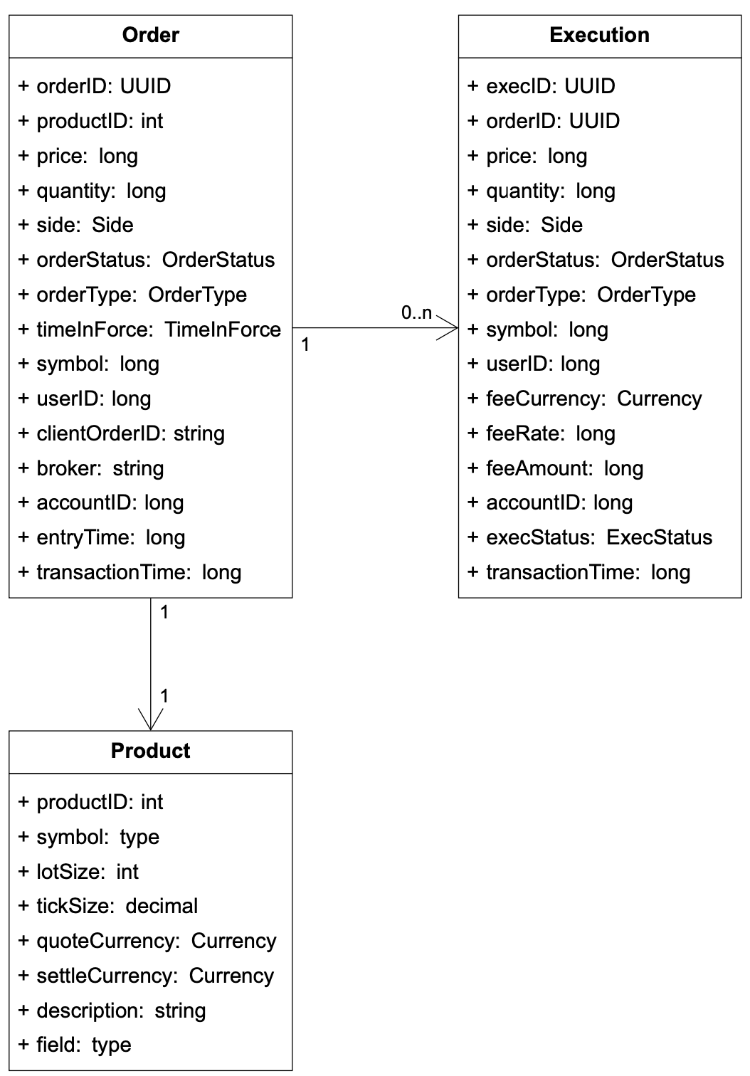
Order book
List of buy/sell orders for a security organized by price level. Key data structure in matching engine.
**Requirements:** O(1) add/cancel/execute, O(1) lookup by price level, fast best-bid/ask query, iterate price levels.
**Implementation:** ``` class PriceLevel { Price limitPrice; long totalVolume; List<Order> orders; } class Book<Side> { Side side; Map<Price, PriceLevel> limitMap; } class OrderBook { Book<Buy> buyBook; Book<Sell> sellBook; PriceLevel bestBid; PriceLevel bestOffer; Map<OrderID, Order> orderMap; } ```
**Key:** Use **doubly-linked list** for `orders` (not plain list) to achieve O(1) for all operations: - **Place** (new order) → append to tail: O(1). - **Match** → delete from head: O(1). - **Cancel** → use `orderMap` to find order in O(1); doubly-linked list allows deletion without traversal (no need to find previous pointer).
Also used in MDP to reconstruct L1/L2/L3 data from execution stream.
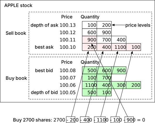
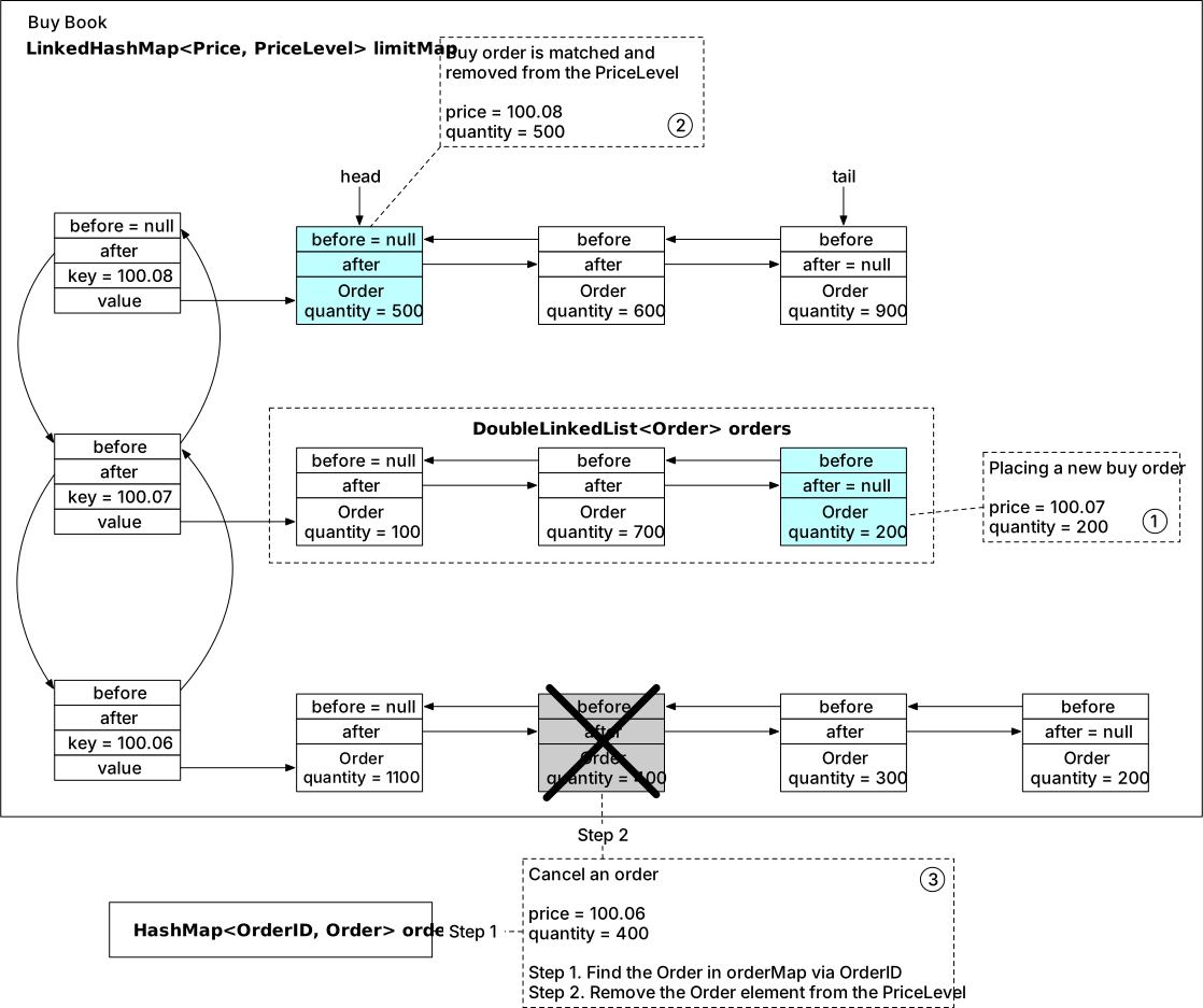
Candlestick chart
Key data structure in MDP alongside order book. ``` class Candlestick { long openPrice; long closePrice; long highPrice; long lowPrice; long volume; long timestamp; int interval; } class CandlestickChart { LinkedList<Candlestick> sticks; } ``` **Memory optimizations:** - Pre-allocated **ring buffers** to hold sticks (no new object allocations). - Limit in-memory sticks; persist the rest to disk.
Market data persisted in **in-memory columnar database** (e.g., KDB) for real-time analytics; historical data persisted to disk after market close.
Step 3 - Design Deep Dive
Modern large exchanges run almost everything on a single gigantic server. Key optimization areas: performance, event sourcing, high availability, fault tolerance.
Performance
`Latency = ∑executionTimeAlongCriticalPath`
**Critical path:** `gateway → order manager → sequencer → matching engine`
**Reduce tasks on critical path:** Even logging is removed from the critical path.
**Reduce time per task — eliminate network and disk access:** - Network round-trip: ~500μs per hop → multiple components = single-digit ms total. - Sequential disk writes (sequencer): tens of ms. - Total: tens of ms — insufficient for modern low-latency exchanges.
**Solution: Put everything on one server (Figure 15).** - Components communicate via **mmap** (`mmap(2)`) over `/dev/shm` (memory-backed filesystem) — no network, no disk I/O. - mmap message bus: sub-microsecond messaging.
**Application loop (Figure 16):** - Single-threaded loop that polls for tasks to execute. - **CPU pinning**: each application loop thread is pinned to a fixed CPU core. - Benefits: no context switch, no lock contention (single writer) → low 99th percentile latency. - Tradeoff: more complex coding; engineers must carefully budget time per task.
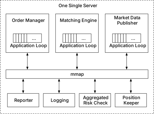
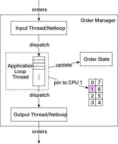
Event sourcing
**Traditional DB approach** (Figure 17 left): stores current state (order status) only — no history of how state was reached.
**Event sourcing** (Figure 17 right): immutable log of all state-changing events. Events are the golden source of truth. State is reconstructed by replaying events.
**Event sourcing design with mmap (Figure 18):** - External domain uses FIX; internal domain uses FIX over SBE (Simple Binary Encoding) for compact/fast encoding. - Gateway transforms FIX → SBE → sends `NewOrderEvent` via Event Store Client. - Order manager (embedded in matching engine): receives `NewOrderEvent`, validates, updates internal order states, sends to matching core. - Matching engine generates `OrderFilledEvent` → event store. - MDP and reporter subscribe to event store.
**Order manager as library:** Embedded in each component that needs order state. Each component maintains its own order state — no shared order manager to avoid latency hit. Event sourcing guarantees all states are identical and replayable.
**Sequencer in event sourcing design (Figure 19):** - Single writer — only one sequencer per event store (multiple would cause lock contention). - Pulls events from each component's local ring buffer, stamps sequence ID, sends to event store. - Simple and fast (no message store function — just stamps IDs). - Backup sequencers for HA.
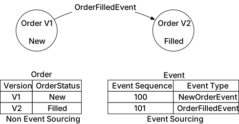
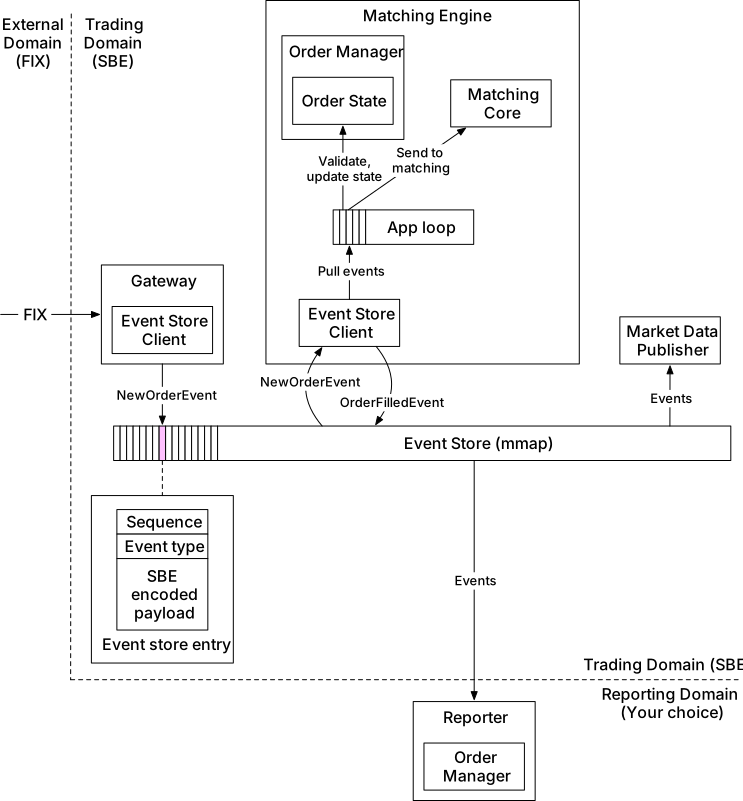
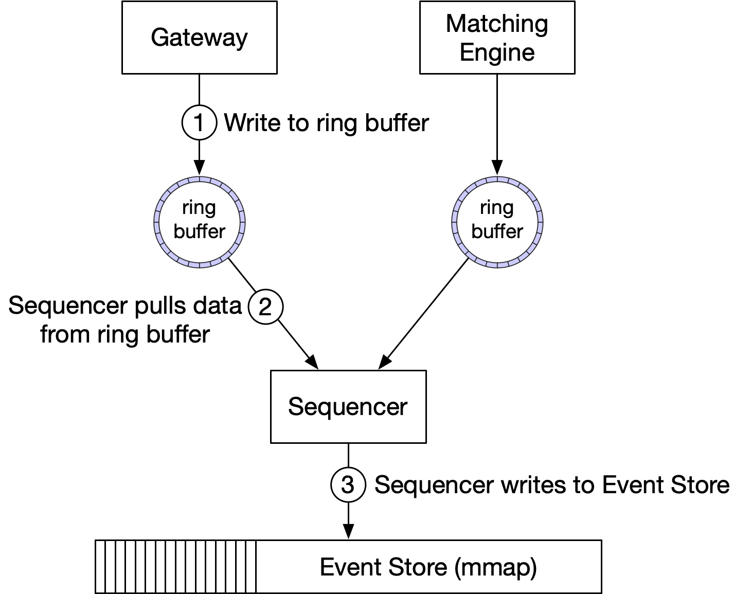
High availability
Goal: 4 nines (99.99%) = max 8.64 seconds downtime/day → immediate recovery required.
**Hot-warm design (Figure 20):** - **Hot (primary) matching engine**: active; sends events to event store. - **Warm (backup) instance**: receives and processes the same events but does not send events out. - On primary failure: warm instance immediately takes over as primary. - On warm failure/restart: recovers all states by replaying event store.
**Heartbeats**: matching engine sends heartbeats; missing heartbeat triggers failover check.
**Scaling hot-warm across machines:** Replicate entire event store across machines and data centers using **reliable UDP** for efficient broadcast to all warm servers (see Aeron design).
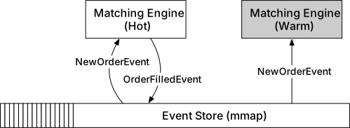
Fault tolerance
Hot-warm design with cross-datacenter replication for disaster recovery (earthquake, power outage).
**Key questions:** - **RTO** (Recovery Time Objective): second-level → requires automatic failover + service degradation strategy. - **RPO** (Recovery Point Objective): near zero data loss → Raft guarantees many copies with consensus.
**Leader election with Raft (Figure 21 & 22):** - 5-node Raft cluster; each node has its own mmap event store. - Leader sends events to all followers over RPC; followers save to their event stores. - Minimum votes to perform operation: N/2 + 1 (3 of 5). - **Heartbeat**: leader sends `AppendEntries` (no content) to followers. - **Election timeout**: follower becomes candidate if no heartbeat received; sends `RequestVote` to others. - First follower with majority votes wins; if tie → split vote → new election. - **Term** (Figure 22): time divided into arbitrary intervals representing normal operation vs. election.
**Failure handling guidance:** - Start with manual failover; automate only after gathering enough operational signals. - Use **chaos engineering** to surface edge cases faster.
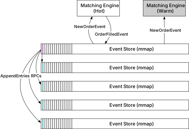
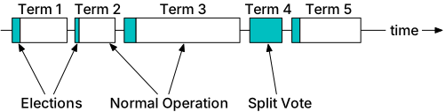
Matching algorithms
Default: **FIFO matching** — orders at the same price level matched in arrival order.
**Other algorithms (used in futures trading):** - **FIFO with LMM (Lead Market Maker)**: pre-allocates a ratio to the LMM ahead of FIFO queue. - **Dark pool**: alternative trading system with different matching rules.
**Pseudocode highlights:** - `handleOrder`: validates sequence ID, validates order, dispatches to `handleNew` or `handleCancel`. - `handleNew`: routes to `match(sellBook, order)` for BUY or `match(buyBook, order)` for SELL. - `handleCancel`: uses `orderMap` to find order; removes and sets CANCELED status. - `match`: iterates doubly-linked list at price level, fills from head until `leavesQuantity == 0`.
Determinism
**Functional determinism**: same input sequence → same output (enabled by sequencer + event sourcing).
**Latency determinism**: stable latency across all trades. Measured by **99th percentile** (or 99.99th) latency using **HdrHistogram**.
**Time in event sourcing (Figure 23)**: actual wall-clock time of events doesn't matter — only ordering matters. Discrete uneven event timestamps converted to continuous sequential dots → replay/recovery time greatly reduced.
**Java latency pitfall**: JVM Stop-the-World GC (HotSpot) causes safe-point pauses — a common source of 99th percentile latency spikes.
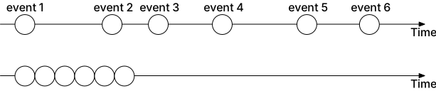
Market data publisher optimizations
MDP receives matched results from matching engine → rebuilds order book and candlestick charts → publishes to subscribers.
**Design uses ring buffers (Figure 24):** - Ring buffer (circular buffer): fixed-size queue with head connected to tail. - Pre-allocated space — no object creation/deallocation. - **Lock-free** data structure. - **Cache line padding**: ensures ring buffer sequence number is never in a cache line with anything else → eliminates false sharing.
**Tiered access:** Retail gets 5 levels of L2 by default; pay extra for more levels.
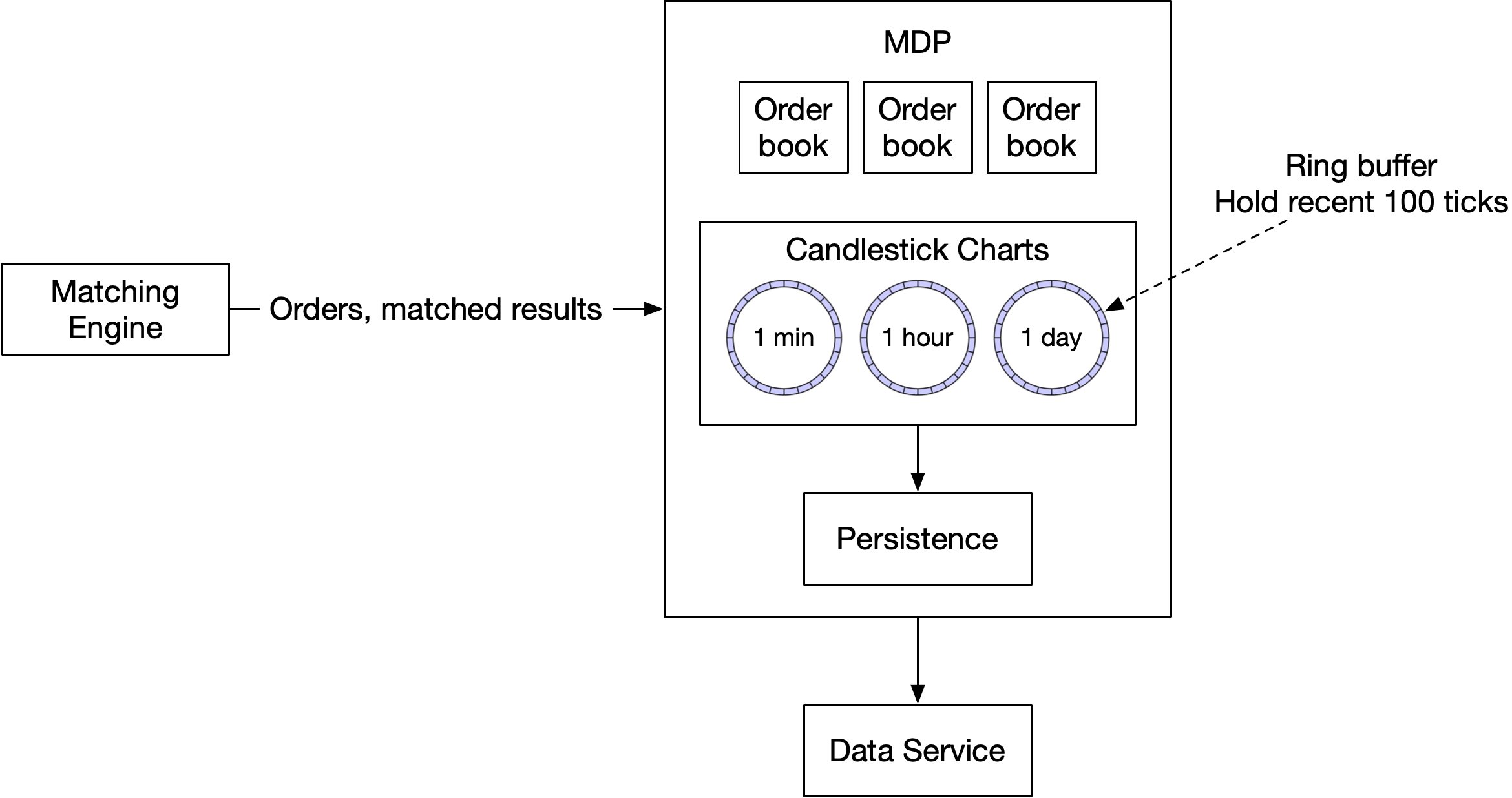
Distribution fairness of market data
For regulated exchanges: all subscribers must receive market data at the same time.
**Problem:** First subscriber in list always receives data first; smart clients race to connect first at market open.
**Solutions:** - **Multicast with reliable UDP**: broadcast updates to many participants simultaneously. - **Random ordering**: assign random position to subscriber on connect.
Multicast
Three data transport protocols: - **Unicast**: one source → one destination. - **Broadcast**: one source → entire subnetwork. - **Multicast**: one source → set of hosts on different subnetworks.
Multicast receivers in the same group receive data simultaneously in theory. UDP is unreliable — use retransmission handling (e.g., NACK-Oriented Reliable Multicast).
Colocation
Exchanges offer colocation services: broker/hedge fund servers placed in the same data center as the exchange. Latency ∝ cable length. Considered a paid VIP service, not a fairness violation.
Network security
DDoS is a real challenge for exchanges with public interfaces.
**Mitigations:** - Isolate public services from private services; multiple read-only copies. - Caching layer for infrequently updated data. - Harden URLs: use `/data/recent` instead of `/data?from=123&to=456` (cacheable at CDN; harder to enumerate). - Safelist/blocklist mechanisms via network gateway products. - **Rate limiting**.
Wrap Up
An ideal deployment for a large exchange: everything on a single gigantic server or single process. Some exchanges are designed exactly this way.
**Crypto exchanges** use cloud infrastructure; some DeFi projects use AMM (Automatic Market Making) without order books entirely.
**Key design topics:** matching engine + sequencer, order book (doubly-linked list O(1)), candlestick charts, client gateway, mmap message bus, application loop with CPU pinning, event sourcing with SBE, hot-warm HA, Raft fault tolerance, FIFO matching, HdrHistogram for latency, ring buffer MDP, multicast for fair data distribution.
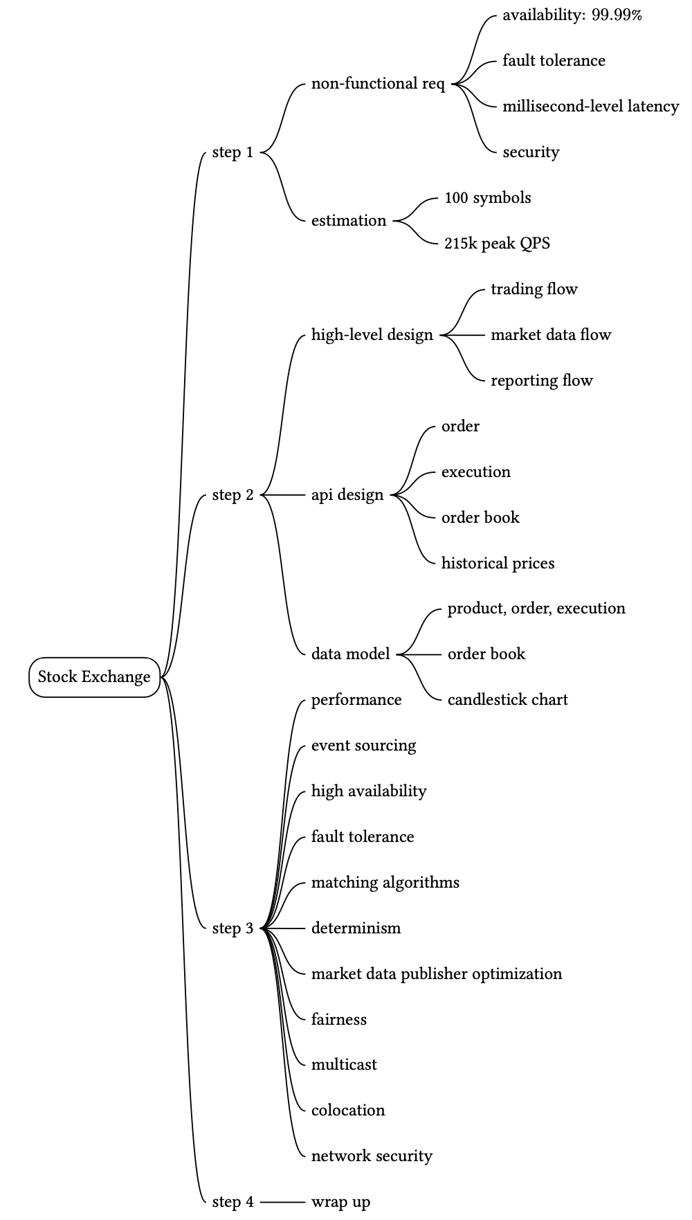
The Learning Continues
Designing good systems requires years of accumulated knowledge. One shortcut is to dive into real-world system architectures. Pay attention to both shared principles and underlying technologies — understand what problems each technology solves.
Real-world systems
Materials covering general design ideas of real system architectures across different companies:
**Facebook** - Facebook Timeline: Brought To You By The Power Of Denormalization - Scale at Facebook - Building Timeline: Scaling up to hold your life story - Erlang at Facebook (Facebook chat) - Finding a needle in Haystack: Facebook's photo storage - Serving Facebook Multifeed: Efficiency, performance gains through redesign - Scaling Memcache at Facebook - TAO: Facebook's Distributed Data Store for the Social Graph
**Amazon** - Amazon Architecture - Dynamo: Amazon's Highly Available Key-value Store
**Netflix** - A 360 Degree View Of The Entire Netflix Stack - It's All A/Bout Testing: The Netflix Experimentation Platform - Netflix Recommendations: Beyond the 5 stars (Part 1 & 2)
**Google** - Google Architecture - The Google File System - Differential Synchronization (Google Docs) - Bigtable: A Distributed Storage System for Structured Data
**YouTube** - YouTube Architecture - Seattle Conference on Scalability: YouTube Scalability
**Twitter** - The Architecture Twitter Uses To Deal With 150M Active Users - Scaling Twitter: Making Twitter 10000 Percent Faster - Timelines at Scale - Announcing Snowflake (unique ID generation at high scale)
**Other** - Instagram Architecture: 14 Million Users, Terabytes Of Photos - How Uber Scales Their Real-Time Market Platform - Scaling Pinterest / Pinterest Architecture Update - A Brief History of Scaling LinkedIn - Flickr Architecture - How We've Scaled Dropbox - The WhatsApp Architecture Facebook Bought For $19 Billion
Company engineering blogs
Reading a company's engineering blog before an interview gives invaluable insight into their tech stack and design decisions.
| Company | Blog | |---------|------| | Airbnb | medium.com/airbnb-engineering | | Amazon | developer.amazon.com/blogs | | Docker | blog.docker.com | | Dropbox | blogs.dropbox.com/tech | | eBay | ebaytechblog.com | | Facebook | code.facebook.com/posts | | GitHub | githubengineering.com | | Google | developers.googleblog.com | | Highscalability | highscalability.com | | Instagram | engineering.instagram.com | | LinkedIn | engineering.linkedin.com/blog | | Netflix | medium.com/netflix-techblog | | PayPal | paypal-engineering.com | | Pinterest | engineering.pinterest.com | | Reddit | redditblog.com | | Shopify | engineering.shopify.com | | Slack | slack.engineering | | Spotify | labs.spotify.com | | Stripe | stripe.com/blog/engineering | | System Design Primer | github.com/donnemartin/system-design-primer | | Twitter | blog.twitter.com/engineering | | Uber | eng.uber.com | | Yelp | engineeringblog.yelp.com | | Zoom | medium.com/zoom-developer-blog |
Congratulations! You are at the end of this interview guide. You have accumulated skills and knowledge to design systems. Practice makes perfect — landing a dream job is a long journey that requires lots of time and effort.